
Section author: Evert Bunschoten
FGM Simulation of a Methane Flame using Tabulated Chemistry#
Important
Documentation in progress!
This tutorial explains how to use SU2 DataMiner to set up the simulation of a premixed methane-air flame using the flamelet-generated manifold (FGM) method in SU2. The thermochemical state variables are retrieved from a two-dimensional look-up table. Instructions on how to generate the table can be found in this tutorial.
Important
This tutorial was written and tested on a Linux operating system. If you want to run it on Windows, make sure you replace the file path separator in the python files! The version of SU2 used for this tutorial was 8.5.1. Please make sure you have the correct version when running this tutorial.
Set-up#
In order to run this tutorial, you need a working installation of SU2 DataMiner. Consult the installation instructions for details. Additionally, you will need a two-dimensional look-up table for premixed methane flames. The tutorial on methane tabulation provides all the instructions on how to generate such a table. The simulation is set up through the python script Tutorials->FGM->01_methane_tabulation->04_prepare_SU2_simulation.py. Finally, you need a working installation of SU2, version 8.4.0 or higher.
Step 1: Defining the Problem and Boundary Conditions#
This tutorial shows the 2D simulation of a premixed methane flame at an equivalence ratio of 0.7 and the temperature of the reactants set to 350 Kelvin. The domain is set up as a 2D bunsen burner in which the flame is anchored on an iso-thermal wall. The computational domain with the boundary conditions is shown in the image below.
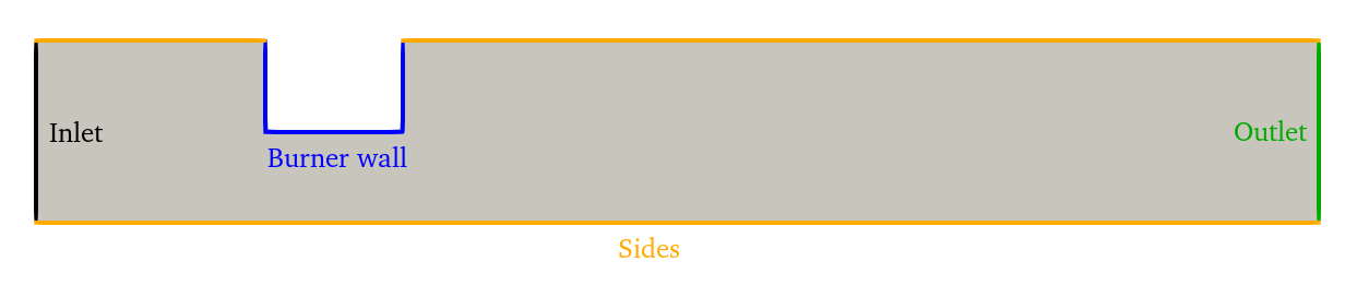
Illustration of the computational domain#
The flow velocity, temperature, and FGM controlling variables are imposed at the inlet boundary. The inflow velocity is calculated to be the laminar flame speed of a methane flamelet with an equivalence ratio of 0.7 and reactant temperature of 300 Kelvin. The following code snippet can be used to calculate the adiabatic flame speed using the configuration generated in the methane tabulation tutorial.
# Reactant temperature and equivalence ratio for simulation
Tu = 350
eq_ratio = 0.7

# Run an adiabatic flamelet simulation to estimate adiabatic flame speed.
config = Config_FGM("methane_tabulation.cfg")
freeflame = FreeFlameSolver(config)
freeflame.setReactantTemperature(Tu)
freeflame.setMixtureStatus(eq_ratio)
freeflame.startSolver()
solution = freeflame.getThermoChemicalData()

flame_velocity = solution["Velocity"].iloc[0]
Step 2: Generating the Computational Grid#
The next step is to generate the computational mesh. The computational domain is sized based on the flame thickness. The dimensions of the computational domain are visualized below.
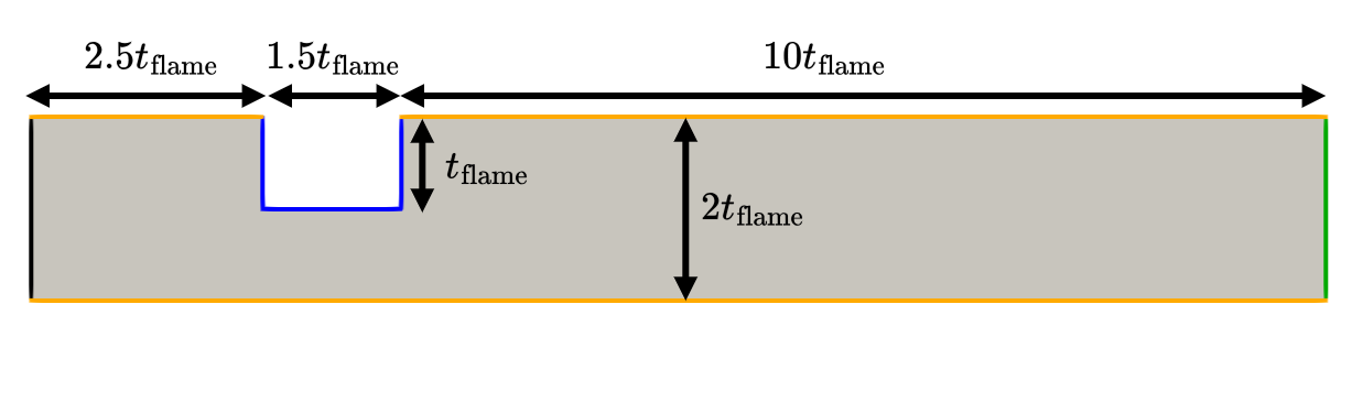
Size of the computational domain with respect to the flame thickness.#
The flame thickness can be calculated through
using the following code snippet:
grid = np.array(solution["Distance"])
dx = grid[1:]-grid[:-1]
T = np.array(solution["Temperature"])
dTdx = (T[1:] - T[:-1])/dx
max_dTdx = max(dTdx)
t_flame = (max(T) - min(T))/max_dTdx
The computational domain is discretized with cells of the same size. The mesh resolution is based on the resolution of the 1D solution.
cell_size = 10*min(dx)
The mesh in this tutorial is generated using Gmesh using the code snippet below:
# Generate mesh
gmsh.initialize()
gmsh.model.add("2D flame domain")
gmsh.option.setNumber("General.Verbosity", 0)
gmsh.option.setNumber("Mesh.MeshSizeFromPoints",0)
gmsh.option.setNumber("Mesh.MeshSizeExtendFromBoundary",0)
gmsh.option.setNumber("Mesh.MeshSizeMax",cell_size)
gmsh.option.setNumber("Mesh.Algorithm", 8)
gmsh.option.setNumber("Mesh.SaveAll",0)
gmsh_geo = gmsh.model.geo
gmsh_mesher = gmsh.model.mesh

x_inlet = -4*t_flame
x_outlet = 10*t_flame
w_domain = 2*t_flame
dx_burner = 1.5*t_flame

pts_inlet = [gmsh_geo.addPoint(x_inlet, 0, 0), gmsh_geo.addPoint(x_inlet, w_domain, 0)]

pts_burner_wall = [gmsh_geo.addPoint(-dx_burner, w_domain, 0),\
                gmsh_geo.addPoint(-dx_burner, 0.5*w_domain, 0),\
                gmsh_geo.addPoint(0, 0.5*w_domain, 0),\
                gmsh_geo.addPoint(0, w_domain, 0)]

pts_outflow = [gmsh_geo.addPoint(x_outlet, w_domain, 0), gmsh_geo.addPoint(x_outlet, 0, 0)]

line_inlet = gmsh_geo.addLine(pts_inlet[0],pts_inlet[1])
lines_burner_wall = [gmsh_geo.addLine(pts_burner_wall[0],pts_burner_wall[1]),\
                    gmsh_geo.addLine(pts_burner_wall[1],pts_burner_wall[2]),\
                    gmsh_geo.addLine(pts_burner_wall[2],pts_burner_wall[3])]

line_outlet = gmsh_geo.addLine(pts_outflow[0],pts_outflow[1])
lines_sym = [gmsh_geo.addLine(pts_inlet[1], pts_burner_wall[0]),\
            gmsh_geo.addLine(pts_burner_wall[-1], pts_outflow[0]),\
            gmsh_geo.addLine(pts_outflow[1], pts_inlet[0])]

crvloop = gmsh_geo.addCurveLoop([line_inlet] + lines_sym + lines_burner_wall+[line_outlet],reorient=True)
fluid_plane = gmsh_geo.addPlaneSurface([crvloop])

gmsh_geo.addPhysicalGroup(1, [line_inlet],name="inlet")
gmsh_geo.addPhysicalGroup(1, [line_outlet],name="outlet")
gmsh_geo.addPhysicalGroup(1, lines_burner_wall,name="burner_wall")
gmsh_geo.addPhysicalGroup(1, lines_sym,name="symmetry")
gmsh_geo.addPhysicalGroup(2, [fluid_plane],name="fluid")

gmsh_geo.synchronize()
gmsh_mesher.setRecombine(2, fluid_plane)
gmsh_mesher.generate(2)
gmsh.write("su2mesh.su2")
gmsh.finalize()
The image below shows a section of the computational mesh generated for this tutorial. After generating the mesh, it is saved locally as the file su2mesh.su2.
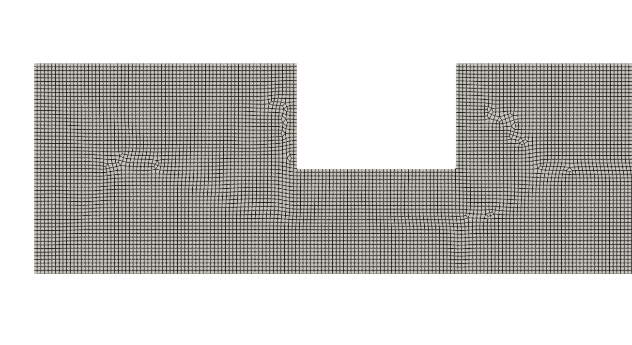
Close-up of the computational mesh near the burner wall.#
Step 3: Writing the SU2 Configuration File#
The final step needed before running the SU2 FGM simulation in this tutorial is to write the SU2 configuration file. This section will explain what each of the various settings in the configuration file do.
The flow regime is incompressible, laminar flow, so the incompressible Navier-Stokes solver is used and turbulence is disabled. .. code-block:
SOLVER = INC_NAVIER_STOKES
KIND_TURB_MODEL= NONE
The following settings describe the themochemical model SU2 uses to calculate fluid properties during the simulation.
The setting FLUID_MODEL=FLUID_FLAMELET tells SU2 to enable the FGM solver. By setting the viscosity model, conductivity model, and diffusivity model to FLAMELET, these quantities are retrieved from the look-up table during the simulation.
By using INC_DENSITY_MODEL=VARIABLE, the fluid density is calculated with the ideal gas law in which the gas constant is calculated with the local value of the mean molecular weight.
FLUID_MODEL= FLUID_FLAMELET
VISCOSITY_MODEL= FLAMELET
CONDUCTIVITY_MODEL= FLAMELET
DIFFUSIVITY_MODEL= FLAMELET

INC_DENSITY_MODEL= VARIABLE
INC_ENERGY_EQUATION = YES
THERMODYNAMIC_PRESSURE= 101325
INC_NONDIM= DIMENSIONAL
The next settings are used to define the FGM model. In this case, the FGM retrieves thermochemical state information from a look-up table, which can be generated by following the steps in this tutorial.
Preferential diffusion is disabled as the data in the look-up table were generated without accounting for preferential diffusion as well.
SU2 will simulate the transport of the FGM controlling variables and passive species. In this case, the controlling variables are the progress variable and the total enthalpy.
The names listed in CONTROLLING_VARIABLE_NAMES should correspond to those in the look-up table file.
Of the controlling variables, only the progress variable has a non-zero source term. If any transported scalars do not have any source terms, the source term should be named NULL or ZERO.
The passive species are listed under USER_SCALAR_NAMES. The source terms of passive species are calculated using
in which \(\dot{\omega}^+\) and \(\dot{\omega}^-\) are the positive and negative source terms, respectively. The negative source term is multiplied with the local value of the scalar \(Y_i\).
For species like CO, this method improves accuracy. For each of the passive species, the names of the variables in the look-up table for the positive and negative source terms are listed sequentially under USER_SOURCE_NAMES.
If species are modeled only with a source term with a single component, such as CO2, only supply the respecitve net source term and set the negative source term to NULL.
Finally, the values of the transported scalars can be clipped to prevent non-physical effects from occurring such as negative values for mass fractions.
KIND_SCALAR_MODEL= FLAMELET
INTERPOLATION_METHOD= LUT
FILENAMES_INTERPOLATOR= (LUT_methane.drg)
PREFERENTIAL_DIFFUSION= NO

CONTROLLING_VARIABLE_NAMES= (ProgressVariable, EnthalpyTot)
CONTROLLING_VARIABLE_SOURCE_NAMES= (ProdRateTot_PV, NULL)
USER_SCALAR_NAMES= (Y-CO,Y-CO2)
USER_SOURCE_NAMES= ( Y_dot_pos-CO,  Y_dot_neg-CO, Y_dot_net-CO2, NULL)

SPECIES_CLIPPING= YES
SPECIES_CLIPPING_MAX= 1.0, 1e7, 1.0, 1.0
SPECIES_CLIPPING_MIN= -1.0, -1e7, 0.0, 0.0
The initial condition is defined by the initial velocity field, the temperature, and the values of the FGM controlling variables.
In this tutorial, the initial velocity is set to twice the laminar flame speed such that the velocity field in the area restriction near the burner wall remains nearly constant during the convergence process.
The value of the total enthalpy specified in SPECIES_INIT is overwritten based on the initial value of the temperature.
The initial value of the total enthalpy is calculated through inverse regression of the temperature in the look-up table using a Newton root finding algorithm.
INC_VELOCITY_INIT= (5.014e-01, 0.0, 0.0 )
INC_TEMPERATURE_INIT= 350
SPECIES_INIT = (-8.120e-02, -1.275e+05, 0, 0)
The initial value of the progress variable can be calculated for any equivalence ratio using
pv_init, _,_ = config.GetUnburntScalars(eq_ratio, Tu)
The following settings are used to define the boundary conditions of the simulation. The inlet is defined as an incompressible velocity-type inlet at which the temperature and velocity vector are specified.
In this tutorial, the inlet velocity is set to the laminar flame speed calculated earlier. In addition to the velocity and temperature, the values of the FGM controlling variables and passive species (in that order) have to be specified with MARKER_INLET_SPECIES.
In this case, the scalar values at the inlet are the same as the initial condition.
The outlet is defined as a static pressure boundary condition at which the relative static pressure should be specified.
The burner wall is defined as an isothermal wall with a temperature of 350 Kelvin used to anchor the flame. By defining the boundary condition as a strong boundary condition, the solution of the total enthalpy at the boundary is calculated through inverse regression.
INC_INLET_TYPE= VELOCITY_INLET
MARKER_INLET = (inlet, 350, 2.507e-01, 1.0, 0.0, 0.0)
MARKER_INLET_SPECIES = (inlet, -8.120e-02, -1.275e+05, 0, 0)

INC_OUTLET_TYPE= PRESSURE_OUTLET
MARKER_OUTLET= (outlet, 0.0)

MARKER_ISOTHERMAL= (burner_wall, 350)
MARKER_SPECIES_STRONG_BC=(burner_wall)

MARKER_SYM= (symmetry)
If the simulation would be run with only the former settings, the simulation would be that of a cold flow without any flame.
In this tutorial, the flame is ignited by introducing an artificial spark in the flow domain, illustrated in the image below.
When initiating the flame front with an artificial spark, source terms are imposed within a sphere in the domain for a specified number of solver iterations.
Under SPARK_INIT, the location of the center of the spark and the spark radius are specified, followed by the solver iteration at which the spark is initiated and the number of iterations for which the source terms are applied.
The values of the scalar source terms within the spark are specified under SPARK_REACTION_RATES.
FLAME_INIT_METHOD= SPARK
SPARK_INIT= (2.843e-03, 5.687e-04, 0, 5.687e-04, 300, 50)

SPARK_REACTION_RATES= (200, 0, 0, 0)

Location of the artificial spark used to initiate the flame front.#
Next are the numerical settings for the flow solver, scalar solver, and linear solver. For FGM simulations, it is particularly important to set CONV_NUM_METHOD_SPECIES=BOUNDED_SCALAR to improve solver robustness.
NUM_METHOD_GRAD= GREEN_GAUSS
CONV_NUM_METHOD_FLOW= FDS
CONV_NUM_METHOD_SPECIES= BOUNDED_SCALAR
MUSCL_FLOW= YES
MUSCL_SPECIES= YES
SLOPE_LIMITER_FLOW = NONE
SLOPE_LIMITER_SPECIES= NONE
TIME_DISCRE_FLOW= EULER_IMPLICIT
TIME_DISCRE_SPECIES= EULER_IMPLICIT

LINEAR_SOLVER= FGMRES
LINEAR_SOLVER_PREC= ILU
LINEAR_SOLVER_ERROR= 1E-4
LINEAR_SOLVER_ITER=20
Convergence settings
CFL_NUMBER= 50
CFL_ADAPT= NO
ITER=4000

CONV_FIELD = RMS_EnthalpyTot
CONV_RESIDUAL_MINVAL= -10
CONV_STARTITER= 20
Finally, there are the input/output settings for the simulation. In this case, the flow solution and restart file are written every 20 solver iterations.
OUTPUT_WRT_FREQ= 20
LOOKUP_NAMES=(Heat_Release)
SCREEN_OUTPUT = INNER_ITER RMS_PRESSURE RMS_ProgressVariable RMS_EnthalpyTot
HISTORY_OUTPUT = WALL_TIME RMS_RES
VOLUME_OUTPUT = SOLUTION, PRIMITIVE, SOURCE, LOOKUP

MESH_FORMAT= SU2
MESH_FILENAME = su2mesh.su2
OUTPUT_FILES = (RESTART,PARAVIEW_MULTIBLOCK)
TABULAR_FORMAT = CSV
CONV_FILENAME= history
VOLUME_FILENAME= flow