Turbulent Bend with wall functions

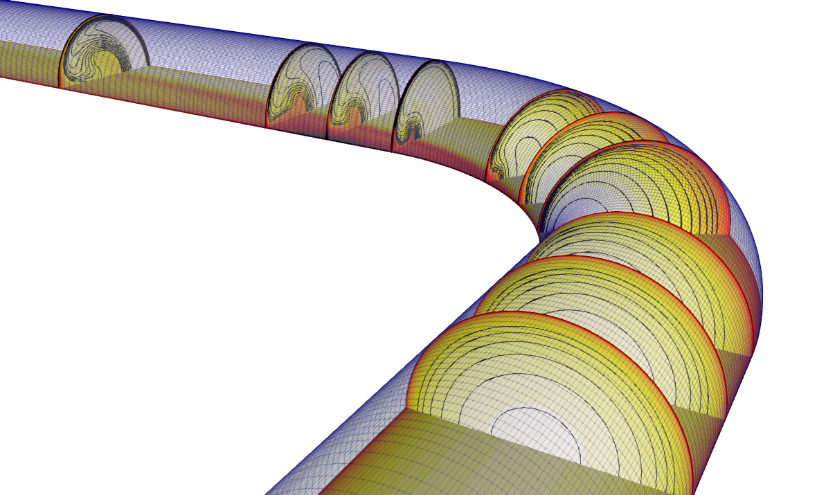
Figure (1): impression of the 90 degree bend with velocity contours.

Goals

In this tutorial we will simulate the turbulent flow in a 90 degree pipe bend. We will touch upon the following aspects:

• the mesh generation in the meshing tool gmsh
• the setup of the model in SU2, using wall functions with the SST turbulence model
• creating a more suitable inlet profile from the solution with uniform inlet conditions
• postprocessing the results with python and paraview

Resources

The resources for this tutorial can be found in the incompressible_flow/Inc_Turbulent_Bend_Wallfunctions directory in the tutorial repository. You will need the configuration file (sudo.cfg) and the mesh file (sudo_coarse.su2). Additionally, the Gmsh geometry is also provided so you can recreate the mesh yourself: sudo_coarse.geo.

This test case was also presented at the 2022 SU2 conference:

• 2022 su2 conference
• doc:Turbulence modeling with wall functions
• youtube:Turbulence modeling with wall functions

Tutorial

The following tutorial will briefly introduce the mesh generation with the meshing software gmsh, which is a great tool especially for structured mesh generation. The test case will then be set up, using wall functions to avoid the use of very fine meshes. The postprocessing with paraview will be briefly introduced, where we do a quick check to see if the solution looks right, and then perform some data extraction for comparison with measurements.

Background

The turbulent flow though the 90 degree circular pipe bend can be seen in Figure 1 and is characterized by 3 flow phenomena that we will try to capture. First of all, the turbulent flow separates in the bend. The exact location depends on the Reynolds number and the radius of curvature of the bend. Secondly, the flow re-attaches after the bend and finally, two counter-rotating vortices are formed after the bend, called Dean vortices. This particular geometry was studied experimentally by Sudo, Sumida and Hibara (Experiments in Fluids 25, 1998) doi and simulation results can be found in Dutta, Saha, Nandi and Pal (Eng. Science Technol. 19(2), 2016) doi.

Problem Setup

The configuration is a 90 degree bend with a diameter of D=0.104 m and a radius of curvature of 2D=0.208 m. We make use of the horizontal symmetry plane and only simulate the upper half of the pipe. The Reynolds number based on pipe diameter is 60,000, which corresponds to a mean velocity of 8.7 m/s. A straight section of L=5D is attached before and a section of L=10D is attached after the bend. Uniform velocity and turbulence boundary conditions are applied at the inlet. The entry length of 5L is not sufficient for turbulence to fully develop and in the experimental setup, the entry and exit lengths were 100D and 40D. This means that the flow conditions that we impose at the inlet are not the actual, fully developed turbulent flow profiles that were present in the experiment. However, This can be solved by first performing a simulation with uniform inlet conditions and then restarting the simulation with an imposed profile for all the transported variables. The inlet profile can be created with paraview from the CFD solution by extracting the solution at 4D downstream of the inlet, where the flow is already partially developed.

Mesh Description

The mesh consists of a structured mesh with 70k cells and 75k points. The mesh was created using Gmsh and the configuration file to create the mesh can be found here: sudo_coarse.geo. The only thing you need to do to create a mesh from the geometry is start Gmsh, and then load the .geo file. You will then see the geometry in the Gmsh visualization window. If you click on Mesh->3D the 3D mesh will be generated. You can then export the mesh as a .su2 file by choosing File->Export. The mesh will automatically be saved in su2 format when the filename has the extension .su2. In general, you should not choose save all elements because this will also save additional points that were used to construct the geometry but are not part of the final mesh, like for example the center of a circle.

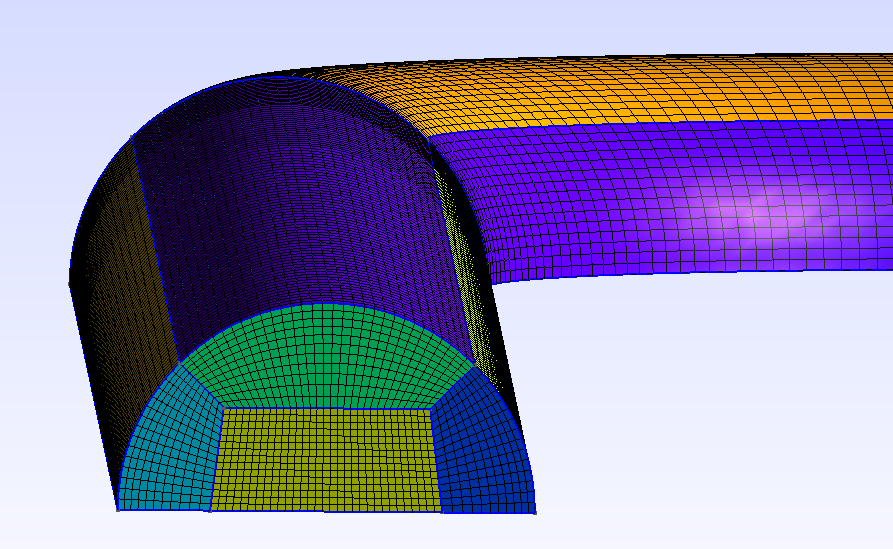
Figure (2): Mesh generated by Gmsh, showing the cross-sectional block structured mesh.

Configuration File Options

Several of the key configuration file options for this simulation are highlighted here. First, we activate the turbulence model:

% ------------- direct, adjoint, and linearized problem definition ------------%
%
SOLVER= INC_RANS
INC_NONDIM= DIMENSIONAL
KIND_TURB_MODEL= SST
SST_OPTIONS= V2003m

We use the incompressible RANS solver to activate the turbulence model and we then choose the SST turbulence model, using the SST_OPTIONS= V2003m variant.

INC_INLET_TYPE= VELOCITY_INLET
INC_OUTLET_TYPE= PRESSURE_OUTLET

The inlet boundary is a velocity inlet and the outlet boundary is a pressure outlet.

MARKER_HEATFLUX= ( wall_1, 0.0, wall_2,0.0, wall_bend,0.0)
MARKER_INLET= ( inlet, 300.0, 8.7, 0.0, 0.0, 1.0 )
MARKER_OUTLET= ( outlet, 0.0)
MARKER_SYM= ( symmetry_1, symmetry_bend, symmetry_2 )
MARKER_INLET_TURBULENT= (inlet, 0.10, 100.0)

There is no heat transfer, so we set zero heatflux boundary conditions on the walls and we impose a velocity of 8.7 m/s, corresponding to the experiment of Sudo et al. The outlet pressure is set to 0 Pa. With the keyword MARKER_INLET_TURBULENT, we set the inlet turbulent intensity and the viscosity ratio. Now we are ready to set up the wall function model:

MARKER_WALL_FUNCTIONS= ( wall_1, STANDARD_WALL_FUNCTION, wall_2,STANDARD_WALL_FUNCTION, wall_bend, STANDARD_WALL_FUNCTION )
WALLMODEL_KAPPA= 0.41
WALLMODEL_B= 5.5
WALLMODEL_MINYPLUS= 1.0
WALLMODEL_MAXITER= 200
WALLMODEL_RELFAC= 0.5

We activate the wall functions with a single option MARKER_WALL_FUNCTIONS. At this moment, the only wall function that you can use is the STANDARD_WALL_FUNCTION. Setting MARKER_WALL_FUNCTIONS is sufficient to set up the wall function model, but there are 5 additional expert options that you can set as well. The constant kappa is interpreted as the von Karman constant and is usually chosen as 0.41. The integration constant B is chosen as 5.5. The minimum value of y+ where the wall function is switched off because the mesh is fine enough to be considered fully resolved is 1.0. A value of 5.0 is the default value chosen in the paper of Nichols and Nelson (2004), but lower values are also possible. Note that Spalding’s fit gives us the nondimensional velocity and therefore the wall shear stress in the entire boundary layer. An iterative process (Newton’s method) is used to compute the nondimensional velocity u+ from y+. The maximum number of iterations chosen here is 200, which is usually more than sufficient. The relaxation factor chosen for the Newton method is 0.5. If you see messages appearing like this:

Warning: computation of wall coefficients (y+) did not converge in 56 points

you can either let the computations continue until the warning messages disappear, increase the maximum number of iterations or decrease the relaxation factor. If these measures do not help, then the problem is most probably due to the mesh quality or due to the physics (flow separation).

Running SU2

If possible, always use a parallel setup to increase computational time. Run the SU2_CFD executable in parallel using MPI and 4 nodes by entering

$ mpirun -n 4 SU2_CFD sudo.cfg

Your results should converge in around 1000 iterations.

Results

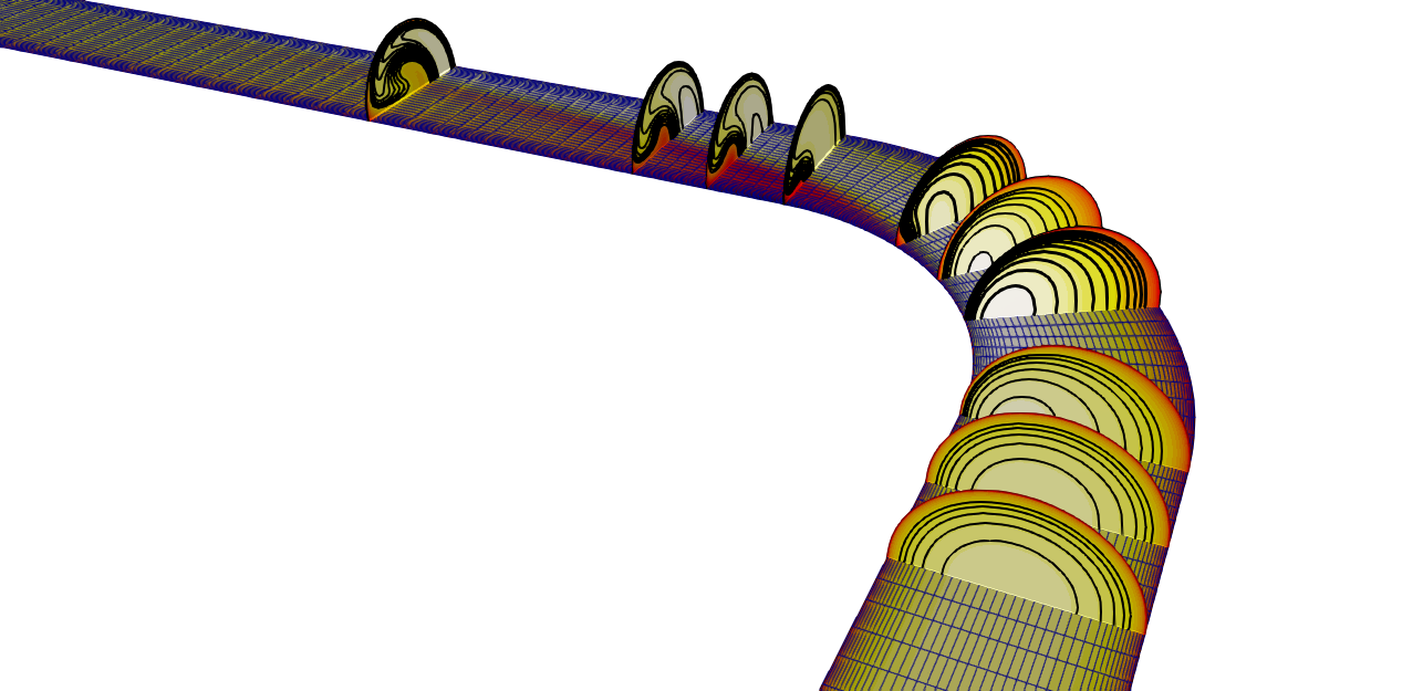Figure (3): Velocity contour with location of the slices where experimental values were obtained.

The paraview multiblock file can now be visualized, and the result is shown in Figure (3). Shown is the velocity magnitude on the horizontal symmetry plane together with a number of contour plots at several vertical locations in the bend.

Part 2 : restart with an inlet profile

In the experiment, the pipe bend was preceded by a very long straight pipe section with a length of 100D, ensuring that the turbulent flow is fully developed by the time it arrives at the pipe bend. In our simulations, we have only a straight section with a total length of 5D and constant inlet properties. We will now restart the simulation with an inlet profile that we extract from a slice of the pipe. It is a planar slice with the normal in the Z-direction, located at Z=2.5D from the inlet. Because in a multiblock mesh, nodes are duplicated on the boundary, so we first perform an Extract Block and select only the interior nodes. We then apply the slice on this extracted block. To keep the original quadrilateral cells, we de-select the option triangulate slice. Also make sure that the option Merge duplicated points in the slice is selected. In the information tab, you should see that the number points is 618, and we will check later that this corresponds with the number of nodes that SU2 expects in the inlet boundary file. Now save the slice data, making sure that only the slice is selected in the Pipeline Browser. Choose the .csv file format, and choose as Arrays To Write only the variables Omega, Pressure, Velocity and Turb_Kin_Energy. The point coordinates are automatically saved. Also choose scientific notation with precision “6” to make sure that you have enough digits for the accurate interpolation of the inlet profile. A simple pvpython script is provided in the tutorials folder here: paraview_extract_slice_data.py. This is a python script that you can run with paraview’s pvpython command and it will generate an inlet.csv file for you :

$ pvpython paraview_extract_slice_data.py

With python, matlab or a simple awk command it is easy to put the data in the correct format for the SU2 inlet profile. The awk command below reads the file inlet.csv, it assumes that the comma acts as a separator, it skips the first line (the header), and then prints the necessary columns and outputs it in the file inlet_test. We want symmetric data in the y-axis, so we check if the y-coordinate in column 2 is positive, and then we write this data for positive and negative y-coordinates. We write the data into the file inlet_test.

awk -F ',' '(NR>1) {if ($2>0.0) {printf ("%8f \t %8f \t %8f \t %6f \t %6f \t %6f \t %f \t %6f \t %6f \t %6f\n ", -$2,$3,-0.52,300.0, $9, 0.0, 0.0, 1.0, $6, $1);printf ("%8f \t %8f \t %8f \t %6f \t %6f \t %6f \t %f \t %6f \t %6f \t %6f\n ", $2,$3,-0.52,300.0, $9, 0.0, 0.0, 1.0, $6, $1)}}' inlet.csv > inlet_data

Now we setup SU2 to use an inlet boundary file. We change some configuration options. Locate and change the following options in the file:

RESTART_SOL= YES
SPECIFIED_INLET_PROFILE= YES
INLET_FILENAME= inlet.dat

The solution was saved as restart.dat and the filename used for the restart is named solution.dat (locate the option for the filenames in the config file!). You can simply copy the restart.dat file to solution.dat and restart the simulation with the above options. If you restart and the file inlet.dat is not present, SU2 will stop with the message

Looked for: inlet.dat. Created a template profile file with default values named example_inlet.dat You can use this file as a guide for making your own profile specification.

You will now have an example inlet profile saved in the file example_inlet.dat. You can now check that this file has 618 rows of data, for each of the nodes on the inlet plane. We only need the header (the first 5 lines of the file), so you can open the file, copy the first 5 lines, open the file inlet_data and add the 5 lines to the top of the file. You can now save this file as inlet.dat and restart the simulation.

Results

We will now compare the simulation results of the pipe bend with results from the paper of Sudo et al. Some velocity measurements were performed at several locations in the pipe bend, and the location that we will use for comparison are shown in the figure below.

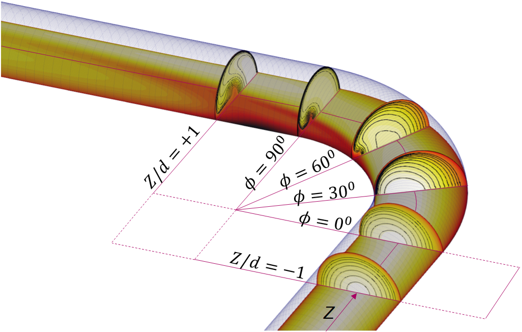
Figure (4): Pipe bend showing the location of the slices that will be used for comparison with measurements.

Below are some of the contour plots taken at several locations in the pipe, showing the velocity normal to the plane with the isocontours in black. The top half are the simulation results and the bottom half are the experimental results from Sudo et al (1998). We see that the main flow features are captured in the simulation.

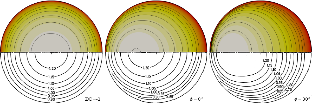
Figure (5): mean flow velocities in several pipe cross sections.

A paraview script to extract the slices data as individual contour plots one by one can be found here: extract_contours_sudo_bend.py.

Below is a comparison of the axial velocity on the horizontal symmetry line through the vertical plane at \(\phi=90^0\). The flow separation in the bend is difficult to capture correctly, and it leads to an underestimation of the local velocity near the inner radius of the bend.

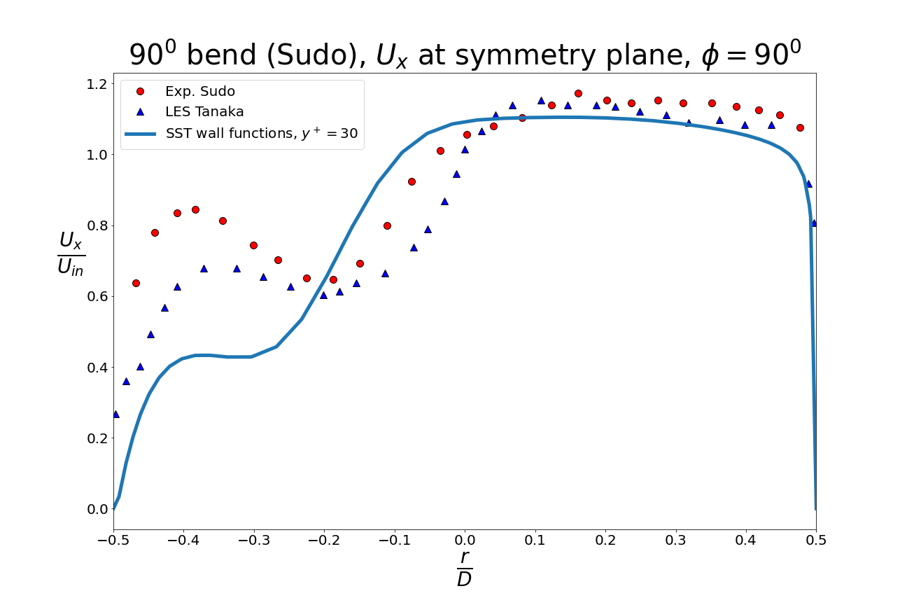
Figure (6): velocity on the symmetry line in the vertical planar cross-section at \(\phi=90^0\).

The paraview script to extract the line data as a .csv file can be found here: paraview_extract_linedata.py