-
Inviscid Bump in a Channel
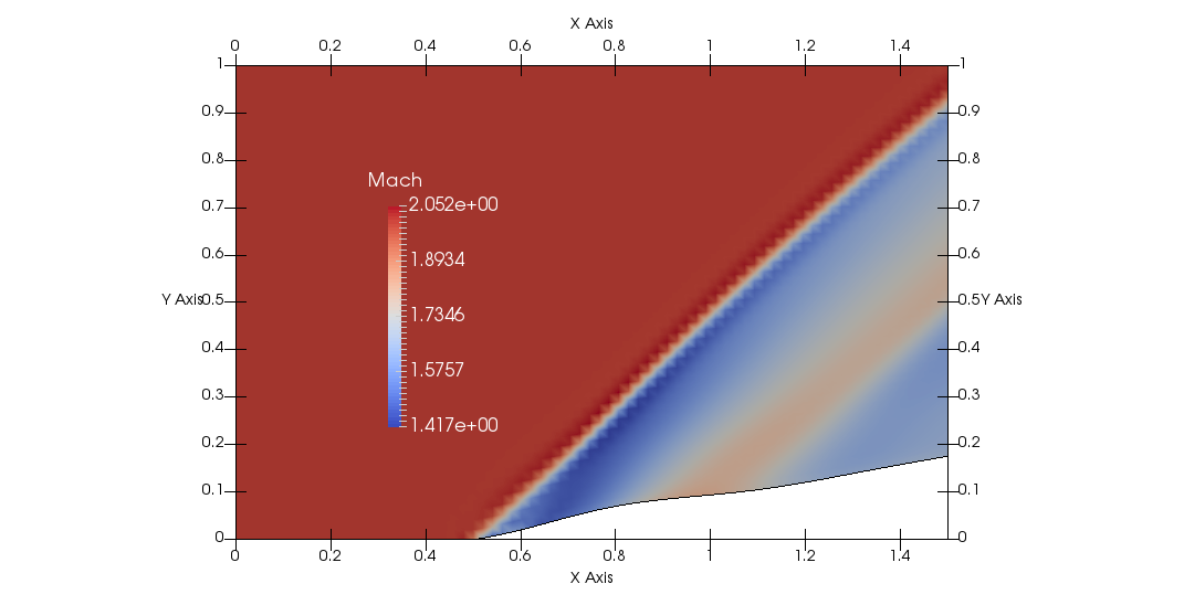
Inviscid Supersonic Wedge
Inviscid ONERA M6
Laminar Flat Plate
Laminar Cylinder
Turbulent Flat Plate
Transitional Flat Plate
Transitional Flat Plate for T3A and T3A-
Turbulent ONERA M6
Unsteady NACA0012
Epistemic Uncertainty Quantification of RANS predictions of NACA 0012 airfoil
Non-ideal compressible flow in a supersonic nozzle
-
Unconstrained shape design of a transonic inviscid airfoil at a cte. AoA
Constrained shape design of a transonic turbulent airfoil at a cte. CL
Constrained shape design of a transonic inviscid wing at a cte. CL
Shape Design With Multiple Objectives and Penalty Functions
Unsteady Shape Optimization NACA0012
Unconstrained shape design of a two way mixing channel
Shape Design With Multiple Objectives and Penalty Functions
| Written by | for Version | Revised by | Revision date | Revised version |
|---|---|---|---|---|
| @hlkline | 7.0.0 | @talbring | 2020-03-03 | 7.0.2 |
Solver: |
|
Uses: |
|
Prerequisites: |
None |
Complexity: |
Advanced |
Goals
Upon completing this tutorial, the user will be familiar with setting up and running an optimization problem that addresses multiple objectives and that uses a penalty function to address a constraint. Consequently, the following capabilities of SU2 will be showcased in this tutorial:
- Multi-objective optimization
- Constraints as penalty functions
- Combining objectives in the adjoint evaluation of the gradient to reduce computational cost.
The intent of this tutorial is to introduce multi-objective, single-point optimization and explain how this can be implemented using SU2. This tutorial uses the same geometry and flow conditions as described in the inviscid supersonic wedge tutorial.
The capabilities of combining multiple objectives and incorporating penalty functions into the adjoint formulation in SU2 are discussed further in section 3.4 of this work.
Resources
The resources for this tutorial can be found in the design/Multi_Objective_Shape_Design directory in the tutorial repository. You will need the configuration file inv_wedge_ROE_multiobj_combo.cfg, the mesh file mesh_wedge_inv_FFD.su2, and solution files solution_flow.csv, solution_adj_combo.csv.
Tutorial
The following tutorial will walk you through the steps required when running a multi-objective optimization problem with SU2. It is assumed you have already obtained or compiled the SU2 executables and python shape optimization scripts. If you have yet to complete these requirements, please see the Download and Installation pages.
Background
Flow Conditions and Mesh Description
The description of the mesh and boundary conditions can be found in the inviscid supersonic wedge tutorial.
Configuration File Options
The configuration file options specifying the boundary conditions Several of the key configuration file options for this simulation are highlighted here. Here we highlight the options required to output one-dimensionalized quantities at a specified marker.
% Outlet boundary marker(s) (NONE = no marker)
% Format: ( outlet marker, back pressure (static), ... )
MARKER_OUTLET= ( outlet, 10000.0 )
...
% Marker(s) of the surface where the functional (Cd, Cl, etc.) will be evaluated
MARKER_MONITORING= (outlet, lower)
...
%
% Marker on which to track one-dimensionalized quantities
MARKER_ANALYZE  = (outlet)
%
% Method to compute the average value in MARKER_ANALYZE (AREA, MASSFLUX).
MARKER_ANALYZE_AVERAGE = AREA
The marker used to track one-dimensionalized quantities must be specified in both MARKER_ANALYZE, and in MARKER_MONITORING. Area averaging, as specified in this example, is used by default. The current verson of the code is only compatible with a single one-dimensionalized marker during optimization.
If we were starting this problem from scratch, at this point it would be prudent to run the CFD simulation in order to check that it is running as expected - the averaged total pressure along with other one-dimensionalized quantities should be output to the history file. With multiple markers specified, integrated quanties such as the drag are the total over all monitored markers, and additional columns are added to the history file showing the per-marker quantities. Next we look at the options used to specify a weighted sum of objectives for the gradient calculation:
% Marker(s) of the surface where the functional (Cd, Cl, etc.) will be evaluated
MARKER_MONITORING= (outlet, lower)
...
% For a weighted sum of objectives: separate by commas, add OBJECTIVE_WEIGHT and MARKER_MONITORING in matching order.
OBJECTIVE_FUNCTION = SURFACE_TOTAL_PRESSURE, DRAG
%
% List of weighting values when using more than one OBJECTIVE_FUNCTION. Separate by commas and match with MARKER_MONITORING.
OBJECTIVE_WEIGHT= -1.0E-7,1.0
These options define a weighted sum: -1.0E-7 x (SURFACE_TOTAL_PRESSURE at the outlet) + (DRAG on the lower surface). The OBJECTIVE_FUNCTION and OBJECTIVE_WEIGHT options are set automatically during the optimization process, and are used for the calculation of the gradient. If we were starting this problem from scratch, at this point we would run the gradient method desired, in order to confirm that the gradients are being calculated as expected. In this tutorial, the discrete adjoint is used by default. When multiple objectives are specified as shown, a single adjoint solution for a ‘combo’ objective will be calculated, representing the gradient for the weighted sum. The upside of this is that it reduces the number of adjoint solutions required, with the downside that the contributions of different functionals to the gradient value will not be known.
Next the FFD box is defined in order to provide the design variables. The mesh is provided with the FFD box information already included, however when starting from scratch a preprocessing step using SU2_MSH is required. For further detail on FFD, see this Unconstrained species transport tutorial or Constrainted Optimal Shape Design Tutorial.
% -------------------- FREE-FORM DEFORMATION PARAMETERS -----------------------%
%
% Tolerance of the Free-Form Deformation point inversion
FFD_TOLERANCE= 1E-10
%
% Maximum number of iterations in the Free-Form Deformation point inversion
FFD_ITERATIONS= 500
%
% FFD box definition: 3D case (FFD_BoxTag, X1, Y1, Z1, X2, Y2, Z2, X3, Y3, Z3, X4, Y4, Z4,
%                              X5, Y5, Z5, X6, Y6, Z6, X7, Y7, Z7, X8, Y8, Z8)
%                     2D case (FFD_BoxTag, X1, Y1, 0.0, X2, Y2, 0.0, X3, Y3, 0.0, X4, Y4, 0.0,
%                              0.0, 0.0, 0.0, 0.0, 0.0, 0.0, 0.0, 0.0, 0.0, 0.0, 0.0, 0.0)
FFD_DEFINITION= (MAIN_BOX, 0.5, -0.25, 0, 1.5, -0.25, 0, 1.5, 0.25,  0, 0.5, 0.25,  0.0, 0.0, 0.0, 0.0, 0.0, 0.0, 0.0, 0.0, 0.0, 0.0, 0.0, 0.0, 0.0, 0.0)
%
% FFD box degree: 3D case (x_degree, y_degree, z_degree)
%                 2D case (x_degree, y_degree, 0)
FFD_DEGREE= (10, 1,0)
%
% Surface continuity at the intersection with the FFD (1ST_DERIVATIVE, 2ND_DERIVATIVE)
FFD_CONTINUITY= 2ND_DERIVATIVE
We will now go over the options necessary to specify the optimization problem. The example below shows settings for a weighted sum of total pressure integrated over the outlet surface and drag evaluated on the solid wall. Note that the order of the objectives matches the order of the markers where they will be evaluated.
In order to optimize for the weighted sum of objectives:
% Optimization objective function with scaling factor, separated by semicolons.
% To include quadratic penalty function: use OPT_CONSTRAINT option syntax within the OPT_OBJECTIVE list.
% ex= Objective * Scale
OPT_OBJECTIVE=SURFACE_TOTAL_PRESSURE*-1E-4; DRAG*1E6
%
% Use combined objective within gradient evaluation: may reduce cost to compute gradients when using the adjoint formulation.
OPT_COMBINE_OBJECTIVE = YES
%
% Optimization constraint functions with scaling factors, separated by semicolons
% ex= (Objective = Value ) * Scale, use '>','<','='
OPT_CONSTRAINT= NONE
%
% Maximum number of iterations
OPT_ITERATIONS= 10
%
% Requested accuracy
OPT_ACCURACY= 1E-6
%
% Upper bound for each design variable
OPT_BOUND_UPPER= 0.1
%
% Lower bound for each design variable
OPT_BOUND_LOWER= -0.1
%
% Optimization design variables, separated by semicolons
DEFINITION_DV= ( 19, 1.0| lower | MAIN_BOX, 3,0,0,1.0);( 19, 1.0| lower | MAIN_BOX, 4,0,0,1.0);( 19, 1.0| lower | MAIN_BOX, 5,0,0,1.0);( 19, 1.0| lower | MAIN_BOX, 6,0,0,1.0)
If OPT_COMBINE_OBJECTIVE is not included or set to ‘NO’, then the gradients will be evaluated separately in sequential operations when adjoint methods are used. Whether to combine the objectives or not will depend on the needs of the problem at hand. If you have a small number of objectives, have plenty of computing resources available, and may need to examine the gradients of the objectives separately from one another, then you may want to forgo combining the objectives and set this option to ‘NO’. On the other hand, if you have a large number of objectives, limited computing resources, and do not need to separate the objective gradients from one another, then combining the objectives may be beneficial.
This tutorial also demonstrates using a penalty function, with the optimization settings shown below. Penalty or barrier functions are functions that increase the magnitude of the objective if it has exceeded a constraint, such that as the optimizer attempts to decrease the magnitude of the objective it is also better satisfying the constraints. In SU2, a quadratic penalty is implemented where if the constraint is violated, the square of the difference between the function value and its constraint is added to the objective. A weighting value is used to scale this function. The syntax for adding a penalty function to the objective is simply to append the same option structure used for OPT_CONSTRAINT to the OPT_OBJECTIVE value, as shown here and in the config file used for this tutorial:
% To include quadratic penalty function: use OPT_CONSTRAINT option syntax within the OPT_OBJECTIVE list.
% ex= Objective * Scale
OPT_OBJECTIVE=AVG_TOTAL_PRESSURE*-1E-4; (DRAG = 0.05)*1E6
%
% Use combined objective within gradient evaluation: may reduce cost to compute gradients when using the adjoint formulation.
OPT_COMBINE_OBJECTIVE = YES
%
% Optimization constraint functions with scaling factors, separated by semicolons
% ex= (Objective = Value ) * Scale, use '>','<','='
OPT_CONSTRAINT= NONE
To use something other than a quadratic penalty, the Python scripts must be modified - specifically SU2_PY/SU2/eval/design.py. As penalty or barrier functions are a somewhat rudimentary method of applying constraints, for some problems the OPT_CONSTRAINT setting will have more success although it requires more gradient evaluations per optimizer iteration. Note that this is only compatible with aerodynamic functions, although geometry-based functions can also be included in the OPT_CONSTRAINT setting.
We will now run the optimization problem, minimizing the total pressure at the outflow surface while constraining the surface drag to equal a specified value.
Running SU2
To run this test case, follow these steps at a terminal command line:
- Move to the directory containing the config file (inv_wedge_ROE_multiobj.cfg) and the mesh file (mesh_wedge_inv_FFD.su2). Make sure that the SU2 tools were compiled, installed, and that their install location was added to your path.
-
Start the optimization by entering
shape_optimization.py -f inv_wedge_multiobj.cfgat the command line. This case will run on a single processor, however the user may want to specify multiple processors using
-n 2appended to the run command for speed. - SU2 will print the combined objective function value and norm of the gradient at each major iteration of the optimizer. While the optimization is running, the progress of each step can be tracked by backgrounding the job or opening another terminal and examining log files in DESIGNS/ subdirectories that are created during this process.
- The optimization history file (history_project.dat) can be visualized in ParaView or Tecplot.
While the optimization problem is running, open the file DESIGNS/DSN_001/ADJOINT_COMBO/config_CFD_AD.cfg. You will need to wait a moment for the initial function evaluation to complete, after which this file will be automatically generated. Search for the ‘OBJECTIVE_FUNCTION’ option to view the adjoint functional specifications. You will see:
OBJECTIVE_FUNCTION= DRAG, SURFACE_TOTAL_PRESSURE
OBJECTIVE_WEIGHT= -11105.0204,0.0001
MARKER_ANALYZE= (outlet)
MARKER_ANALYZE_AVERAGE= AREA
The weight on the SURFACE_TOTAL_PRESSURE function is as specified, and the weight on the drag function is set to the specified weight multiplied by the partial derivative of the penalty function with respect to the drag value, which for the quadratic function used will be 2x(DRAG - 0.05). The sign is determined by whether a ‘>’, ‘<’, or ‘=’ symbol has been used. If the drag meets the specified constraint, the weight will be 0.0.
Results
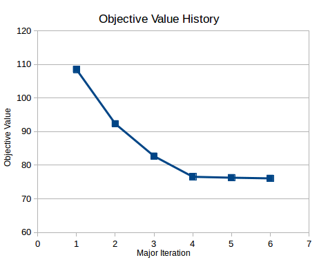
The following images show some results for the supersonic wedge multi-objective optimization problem. After 6 major iterations, and 9 total iterations, the value of the combined objective, which adds a penalty on the total pressure to the value of the drag evaluated on the lower surface of the volume, is seen to approach a constant value. The dashed lines indicate minor iterations taken in between major iterations of the optimizer. The output to the screen should look something like this:
  NIT    FC           OBJFUN            GNORM
    1     1     1.084701E+02     1.504627E+01
    2     2     9.232271E+01     7.491271E+02
    3     4     8.269967E+01     2.792788E+02
    4     5     7.656010E+01     1.854283E+01
    5     7     7.629544E+01     1.679922E+01
    6     9     7.608771E+01     6.110842E+00
Optimization terminated successfully.    (Exit mode 0)
            Current function value: 76.1655658812
            Iterations: 6
            Function evaluations: 20
            Gradient evaluations: 6
The function value listed is the combination of the objective and the penalty function value. Looking at the history of the combined objective, we can see that the combined value has approached a constant value, which is why the optimization problem stopped before reaching the maximum number of iterations.
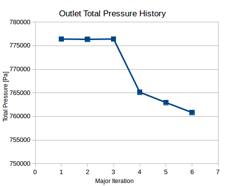
Investigating the history of the total pressure, we can see that the total pressure is still being reduced at the last step, indicating that it could have obtained a lower value if the constraint had not been present, and that the drag value initially oscillates about the specified constraint.
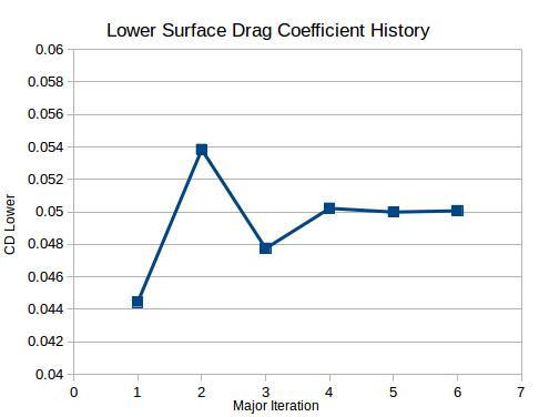
Note that the ‘Cd_lower’ value is plotted rather than ‘DRAG’ because the latter is the total drag over all monitored surfaces.
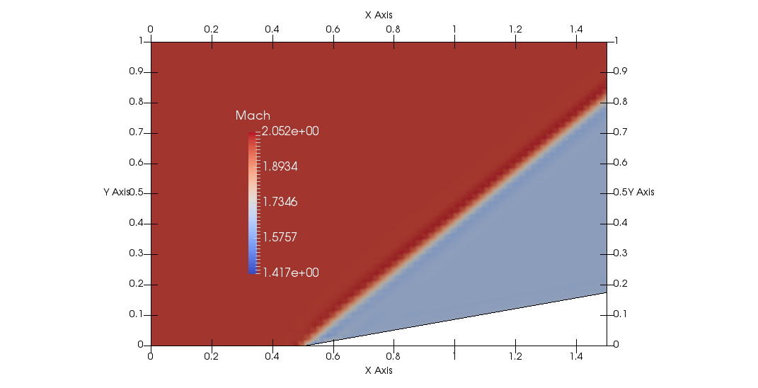
The geometry change to the wedge can be seen in the following figures. The shock structure of the flow has changed in order to approach the constraint and lower the total pressure at the outflow.
Comparison to OPT_COMBINE_OBJECTIVE = NO
By default, objectives are not combined, and when multiple objectives are listed their gradients will be evaluated sequentially. To see the effect of this, first run the tutorial using the files as provided, and track how long it takes to complete on your system. Look in the ‘DESIGNS’ directory, and observe how many subdirectories in the pattern DESIGNS/DSN_*/ADJOINT_* have been generated - there should be one per major iteration. As the next step will overwrite these files, you should rename this directory if you want to save these results.
Next, modify the input file to set ‘OPT_COMBINE_OBJECTIVE = NO’:
% Use combined objective within gradient evaluation: may reduce cost to compute gradients when using the adjoint formulation.
OPT_COMBINE_OBJECTIVE = NO
%
% Optimization constraint functions with scaling factors, separated by semicolons
% ex= (Objective = Value ) * Scale, use '>','<','='
OPT_CONSTRAINT= NONE
%
% Maximum number of iterations
OPT_ITERATIONS= 10
Execute the shape optimization script as before. The problem will most likely take longer to complete. While you are waiting for this problem to complete, open the configuration file generated in DESIGNS/DSN_001/ADJOINT_DRAG/config_CFD_AD.cfg. Search for the OBJECTIVE_FUNCTION option, and you will find that the optimization script has automatically set up the adjoint problem for drag on the lower surface.
Once the optimization problem is completed, you should be able to see that a larger number of subdirectories in the pattern DESIGNS/DSN_*/ADJOINT_* have been generated - this indicates that a larger number of adjoint evaluations were used. You may also notice that the problem will take longer to complete, although the same number of optimizer iterations are used.