Slope Limiters and Shock Resolution
This page lists the limiters available in SU2 and their associated options, it is not meant as a detailed theory guide but a brief review of the governing mathematics is presented. The options listed here do not apply to the high order DG solver.
- Theory: An introduction to slope limiters
- Available Limiter Options
- Empirical comparison of limiters on a periodic advective domain
Theory: An introduction to slope limiters
For many studying compressible flow or high-speed aerodynamics, the formation of shock discontinuities is a common occurrence. The use of high-order numerical schemes is desired to resolve these regions as the strength of the shock largely governs the behavior of the downstream flow field. However, high-resolution linear schemes often result in numerical oscillations near the shock due to the high-frequency content associated with the shock. These oscillations can result in non-physical values (e.g. negative density) that significantly degrade the accuracy of your solution and pollute the domain. An example of this phenomenon is shown below with a MATLAB implementation of the Lax-Wendroff scheme for scalar advection. Although the Lax-Wendroff method is second-order, note that it introduces numerical oscillations that result in the state value of \(u\) becoming negative.
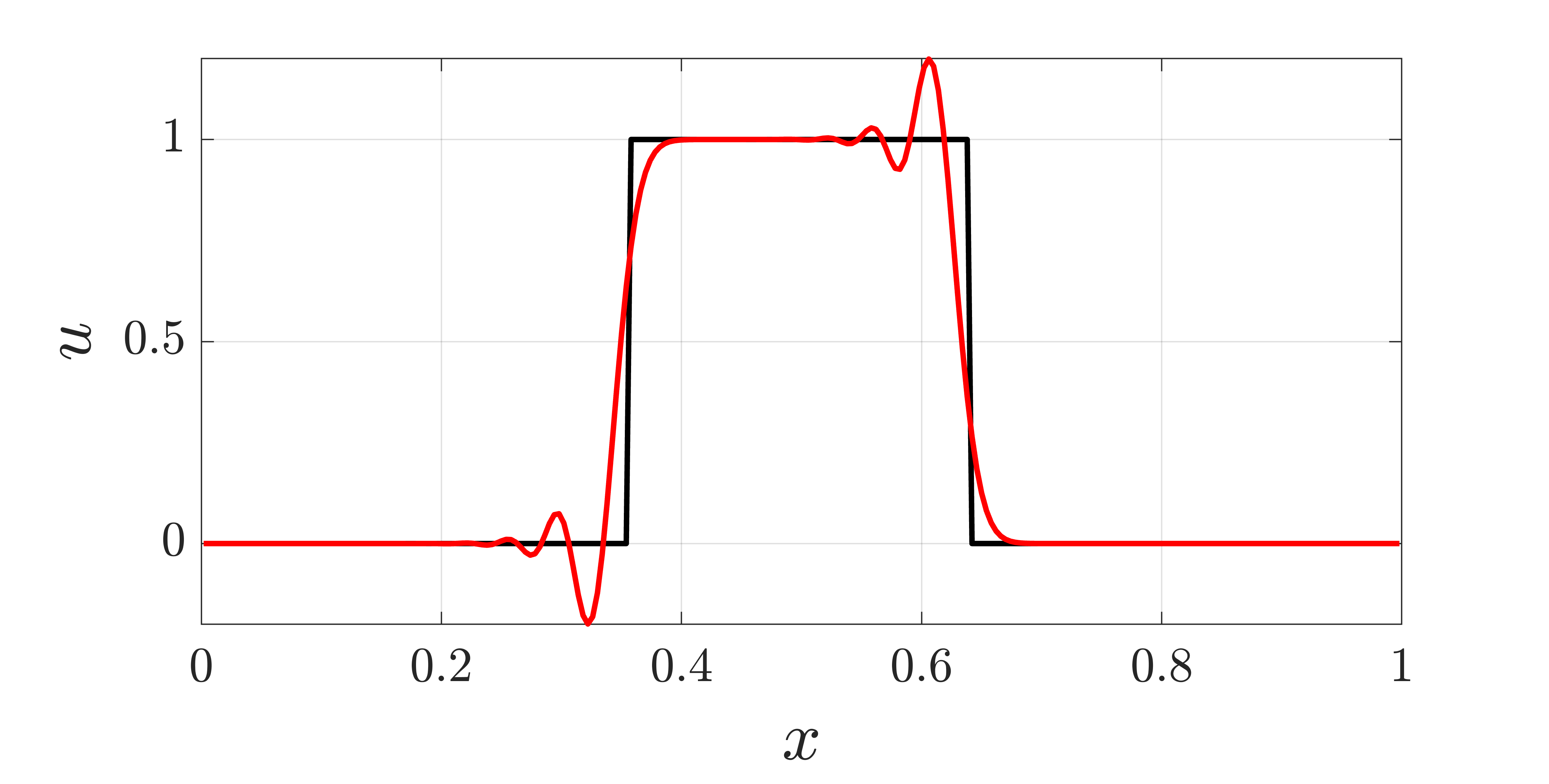
Figure (1): A MATLAB simulation of a one period advection (red) of an initial value discontinuity (black) using the Lax-Wendroff method.
SU2 uses slope limiters to avoid these oscillations by damping second-order terms near shocks and other regions with sharp gradients. The second-order reconstruction is kept where the solution is smooth. This preserves solution accuracy in regions with smooth gradients and helps obtain physical results and numerical stability in regions close to the shock.
Before mathematically describing the form of the limiters implemented in SU2, it is useful to briefly understand two concepts. These include Total Variation and Godunov’s Theorem.
Total Variation and Total Variation Diminishing
We can first introduce the concept of total variation (TV) which is a measure of how oscillatory a solution is. In a discrete one dimensional setting, TV can be calculated as the following:
\[TV(u^n) = \sum_j |u^n_{j+1} - u^n_j|\]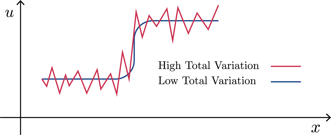
Figure (2): A numerical scheme resulting in both high and low TV.
A scheme can be said to be total variation diminishing (TVD) if
\[TV(u^{n+1}) \leq TV(u^n)\]where for every successive timestep \(n\), the total variation of the solution does not increase.
A favorable property of TVD schemes is that they are monotonicity preserving. This means they do not introduce new extrema into the solution and local minimum (maximum) are non-decreasing (increasing) in time. These are both desirable qualities for correctly resolving a shock and ensuring the solution is physical.
Godunov’s Theorem
The question of “How accurate can a TVD scheme be?” is still unanswered. For this, we turn to Godunov’s Theorem.
Godunov’s Theorem:
- A linear scheme is monotone if and only if it is total variation diminishing.
- Linear total variation diminishing schemes are at most first-order accurate.
The first statement is simple, stating that for linear schemes, the characteristic of being monotone and TVD is equivalent. The second statement is more interesting. It states that if we want to construct a linear TVD (monotone) scheme, the best we can be possibly hope for is first-order accuracy.
Recall that the original motivation for a slope limiter was to prevent the formation of oscillations in the solution. In the section above, we noted that TVD schemes are monotonicity preserving (a favorable property in resolving a shock). However, through Godunov’s theorem, we note that if we also want high-order accuracy, our TVD discretization MUST be nonlinear
The inclusion of a slope limiter into a TVD scheme accomplishes this idea.
Available Limiter Options
The field SLOPE_LIMITER_FLOW in the .cfg file specifies which limiter to use. Note that this option is only used if MUSCL_FLOW = YES (which specifies to use a second-order method).
The Laminar Cylinder shows an example of this.
The Turbulent Flat Plate example sets SLOPE_LIMITER_TURB, which is used for the turbulence equations (if MUSCL_TURB = YES), rather than for the flow equations.
More possible applications of limiters are listed below.
Slope Limiter Fields
| Configuration Field | Description | Notes |
|---|---|---|
SLOPE_LIMITER_FLOW |
Flow equations | Need MUSCL_FLOW = YES |
SLOPE_LIMITER_TURB |
Turbulence equations | Need MUSCL_TURB = YES |
SLOPE_LIMITER_SPECIES |
Species evolution equations | Need MUSCL_SPECIES = YES |
SLOPE_LIMITER_ADJFLOW |
Adjoint flow equations | Need MUSCL_ADJFLOW = YES |
SLOPE_LIMITER_ADJTURB |
Adjoint turbulence equations | Need MUSCL_ADJTURB = YES |
The SLOPE_LIMITER_ options above may each be changed to use different limiters, which are listed and explained below.
Note: the Discontinuous-Galerkin methods (DG) / Higher-order methods (HOM) do not use limiters.
Available Limiters
| Type | Description | Notes |
|---|---|---|
NONE |
No limiter | |
BARTH_JESPERSEN |
Barth-Jespersen | This limiter is a smooth version of the commonly seen Barth-Jespersen limiter seen in the literature |
VENKATAKRISHNAN |
Venkatakrishnan | |
VENKATAKRISHNAN_WANG |
Venkatakrishnan-Wang | |
NISHIKAWA_R3 |
Nishikawa-R3 | |
NISHIKAWA_R4 |
Nishikawa-R4 | |
NISHIKAWA_R5 |
Nishikawa-R5 | |
SHARP_EDGES |
Venkatakrishnan with sharp-edge modification | This limiter should not be used for flow solvers |
WALL_DISTANCE |
Venkatakrishnan with wall distance modification | This limiter should not be used for flow solvers |
VAN_ALBADA_EDGE |
Van Albada (edge formulation) | This limiter is only implemented for flow solvers and does not output limiter values when using the VOLUME_OUTPUT option |
The default limiter is VENKATAKRISHNAN.
Limiter Parameters and Further Details
The VENKAT_LIMITER_COEFF parameter is generally a small constant, defaulting to \(0.05\), but its specific definition depends on the limiter being used.
For the VENKATAKRISHNAN, SHARP_EDGES, and WALL_DISTANCE limiters, the VENKAT_LIMITER_COEFF parameter refers to \(K\) in \(\epsilon^2=\left(K\bar{\Delta} \right)^3\), where \(\bar{\Delta}\) is an average grid size (this is hardcoded as 1m and thus all tuning is via \(K\)). For NISHIKAWA_Rp limiters, \(\epsilon^p=\left(K\bar{\Delta} \right)^{p+1}\) (p = 3, 4 or 5).
The \(K\) parameter defines a threshold, below which oscillations are not damped by the limiter, as described by Venkatakrishnan.
Thus, a large value will approach the case of using no limiter with undamped oscillations, while too small of a value will slow the convergence and add extra diffusion.
The SU2 implementation of the BARTH_JESPERSEN limiter actually uses VENKATAKRISHNAN with \(K=0\).
Note: the value of VENKAT_LIMITER_COEFF depends on both the mesh and the flow variable and thus should be reduced if the mesh is refined.
When using the VENKATAKRISHNAN_WANG limiter, VENKAT_LIMITER_COEFF is instead \(\varepsilon '\) in \(\varepsilon = \varepsilon ' (q_{max} - q_{min})\), where \(q_{min}\) and \(q_{max}\) are the respective global minimum and maximum of the field variable being limited.
This global operation incurs extra time costs due to communication between MPI ranks.
The original work by Wang suggests using VENKAT_LIMITER_COEFF in the range of \([0.01, 0.20]\), where again larger values approach the case of using no limiter.
Note: unlike the aforementioned VENKATAKRISHNAN limiter and NISHIKAWA_Rp limiter, the VENKATAKRISHNAN_WANG limiter does not depend directly on the mesh size and can thus be used without non-dimensionalization. If the VENKATAKRISHNAN limiter is used outside of non-dimensional mode, the fields with larger values (pressure and temperature) will generally be limited more aggressively than velocity.
The NONE, BARTH_JESPERSEN, VENKATAKRISHNAN, VENKATAKRISHNAN_WANG, and NISHIKAWA_Rp limiter options all have no geometric modifier.
A geometric modifier increases limiting near walls or sharp edges. This is done by multiplying the limiter value by a geometric factor.
For both the SHARP_EDGES and WALL_DISTANCE limiters, the influence of the geometric modifier is controlled with ADJ_SHARP_LIMITER_COEFF which defaults to 3.0.
Note: these limiters should not be used for flow solvers, as they only apply to the continuous adjoint solvers.
Increasing this parameter will decrease the value of the limiter and thus make the field more diffusive and less oscillatory near the feature (sharp edge or wall).
In the SHARP_EDGES limiter, the qualification of what makes an edge “sharp” is described by the parameter REF_SHARP_EDGES (defaults to 3.0). Increasing this will make more edges qualify as “sharp”.
Other than the addition of this geometric factor, these limiters are the same as the VENKATAKRISHNAN limiter and should also use VENKAT_LIMITER_COEFF (given by \(K\) below).
Specifically, given the distance to the feature, \(d_{\text{feature}}\), an intermediate measure of the distance, \(d\), is calculated. The parameter \(c\) is set by ADJ_SHARP_LIMITER_COEFF.
Then, the geometric factor is given by
\[\gamma (d) = \frac{1}{2} (1+d+\sin(\pi \cdot d)/ \pi)\]Note that the geometric factor is nonnegative and nondecreasing in \(d_{feature}\).
After the number of iterations given by LIMITER_ITER (default \(999999\)), the value of the limiter will be frozen.
The option FROZEN_LIMITER_DISC tells whether the slope limiter is to be frozen in the discrete adjoint formulation (default is NO).
Empirical comparison of limiters on a periodic advective domain
An example problem of the linear advection problem against four unique wave-forms was simulated in MATLAB to illustrate differences between the primary limiters in SU2. The wave forms contain both smooth and discontinuous initial conditions and are advected for a single period with a CFL of \(\sigma = 0.8\). The domain is discretized with \(N = 200\) cells. The Lax-Wendroff scheme was used as a comparative case:
\[u_j^{n+1} = u_j^{n} - \sigma (u_j^{n} - u_{j-1}^{n}) - \frac{1}{2}\sigma(1-\sigma) \left[ \phi_{j+\frac{1}{2}}(u_{j+1}^{n} - u_j^{n}) - \phi_{j-\frac{1}{2}}(u_{j}^{n} - u_{j-1}^{n}) \right]\]where \(\phi_{j+\frac{1}{2}}\) is the scalar value of the limiter at the interface of cell \(u_j\) and \(u_{j+1}\).
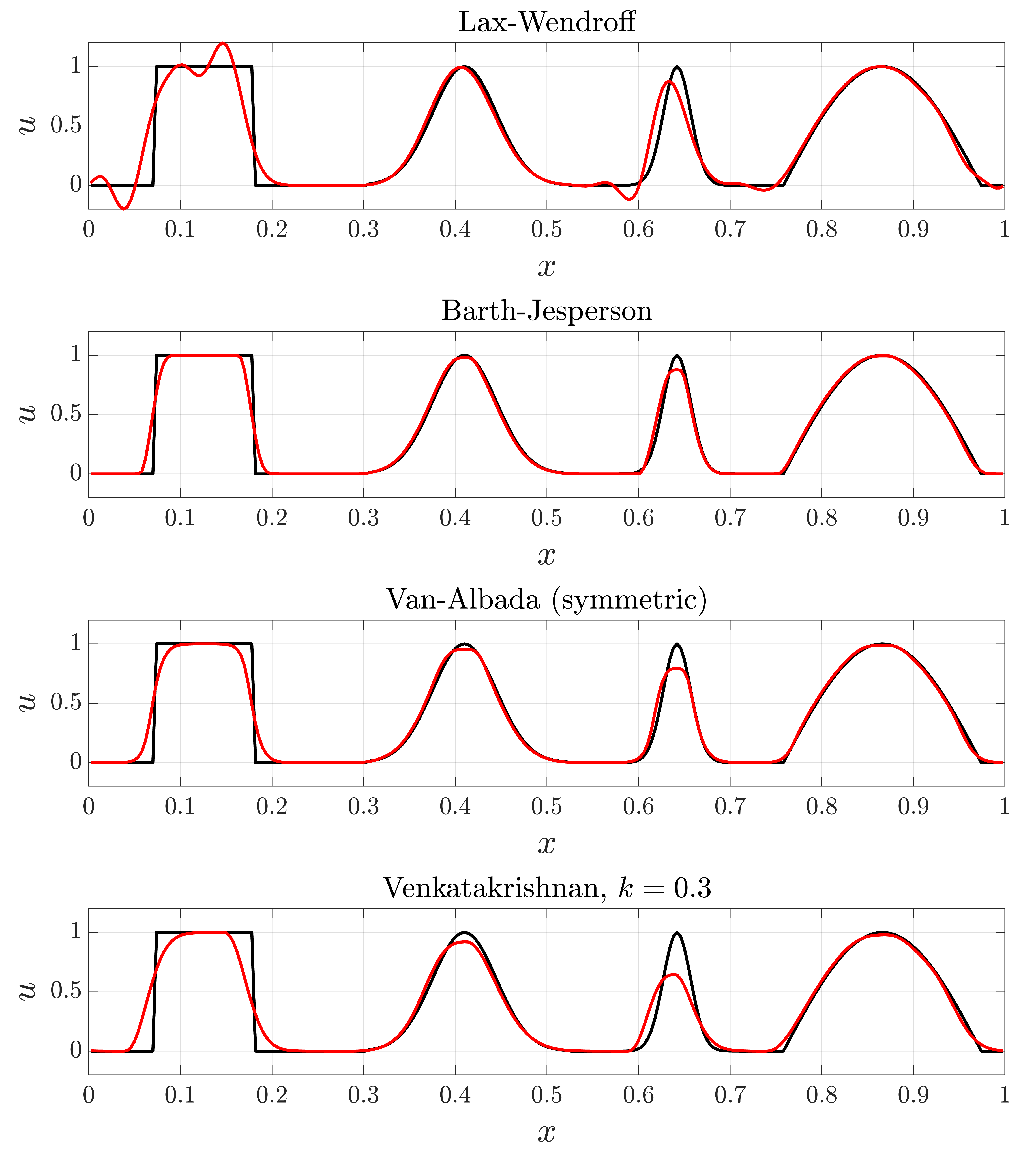
Figure (3): A MATLAB simulation of one period advection (red) of an initial condition (black) using various schemes, with and without limiters.
From the above example we note:
- The Lax-Wendroff scheme produces oscillations near sudden gradients due to dispersion errors. From Godunov’s theorem this is expected as the scheme is second-order accurate and does not utilize a limiter.
- The Barth-Jespersen limiter performs well for most of the waveforms. However, the Barth-Jespersen limtier is known to be compressive and will turn smooth waves into square waves. This is best seen with the value discontinuity on the very left.
- The Van-Albada limiter also performs well. It is slightly more diffusive than Barth-Jespersen but has robust convergence properties.
- The Venkatakrishnan limiter is similar to the Barth-Jespersen and has significantly improved convergence properties. However, it is more diffusive and does require a user-specified parameter \(K\) that is flow dependent.