Solver Setup
This is a basic introduction on how to set up a simulation using SU2. We distinguish between single-zone computations and multi-zone computations. The following considers a single zone only. For an explanation on multi-zone problems, continue with Basics of Multi-Zone Computations.
Defining the Problem
| Solver | Version |
|---|---|
ALL |
7.0.0 |
SU2 is capable of dealing with different kinds of physical problems. The kind of problem is defined by choosing a solver using the SOLVER option. A list of possible values and a description can be found in the following table:
| Option Value | Problem | Type |
|---|---|---|
EULER |
Euler’s equation | Finite-Volume method |
NAVIER_STOKES |
Navier-Stokes’ equation | Finite-Volume method |
RANS |
Reynolds-averaged Navier-Stokes’ equation | Finite-Volume method |
NEMO_EULER |
Thermochemical Nonequilibrium Euler’s equation | Finite-Volume method |
NEMO_NAVIER_STOKES |
Thermochemical Nonequilibrium Navier-Stokes’ equation | Finite-Volume method |
INC_EULER |
Incompressible Euler’s equation | Finite-Volume method |
INC_NAVIER_STOKES |
Incompressible Navier-Stokes’ equation | Finite-Volume method |
INC_RANS |
Incompressible Reynolds-averaged Navier-Stokes’ equation | Finite-Volume method |
HEAT_EQUATION_FVM |
Heat equation | Finite-Volume method |
ELASTICITY |
Equations of elasticity | Finite-Element method |
FEM_EULER |
Euler’s equation | Discontinuous Galerkin FEM |
FEM_NAVIER_STOKES |
Navier-Stokes’ equation | Discontinuous Galerkin FEM |
MULTIPHYSICS |
Multi-zone problem with different solvers in each zone | - |
Every solver has its specific options and we refer to the tutorial cases for more information. However, the basic controls detailed in the remainder of this page are the same for all problems.
Restarting the simulation
| Solver | Version |
|---|---|
ALL |
7.0.0 |
A simulation can be restarted from a previous computation by setting RESTART_SOL=YES. If it is a time-dependent problem, additionally RESTART_ITER must be set to the time iteration index you want to restart from:
% ------------------------- Solver definition -------------------------------%
%
% Type of solver
SOLVER= EULER
%
% Restart solution (NO, YES)
RESTART_SOL= NO
%
% Iteration number to begin unsteady restarts (used if RESTART_SOL= YES)
RESTART_ITER= 0
%
Controlling the simulation
| Solver | Version |
|---|---|
ALL |
7.0.0 |
A simulation is controlled by setting the number of iterations the solver should run (or by setting a convergence critera). The picture below depicts the two types of iterations we consider.
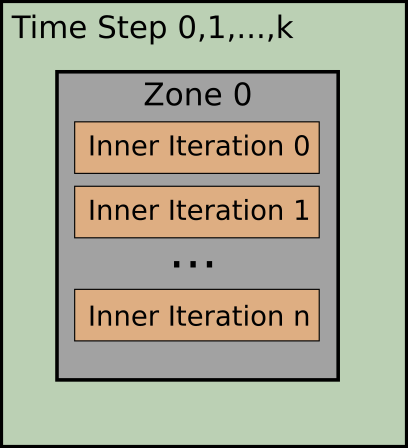
SU2 makes use of an outer time loop to march through the physical time, and of an inner loop which is usually a pseudo-time iteration or a (quasi-)Newton scheme. The actual method used depends again on the specific type of solver.
Time-dependent Simulation
| Solver | Version |
|---|---|
ALL |
7.0.0 |
To enable a time-dependent simulation set the option TIME_DOMAIN to YES (default is NO). There are different methods available for certain solvers which can be set using the TIME_MARCHING option. For example for any of the FVM-type solvers a first or second-order dual-time stepping (DUAL_TIME_STEPPING-1ST_ORDER/DUAL_TIME_STEPPING-2ND_ORDER) method or a conventional time-stepping method (TIME_STEPPING) can be used.
% ------------------------- Time-dependent Simulation -------------------------------%
%
TIME_DOMAIN= YES
%
% Time Step for dual time stepping simulations (s)
TIME_STEP= 1.0
%
% Total Physical Time for dual time stepping simulations (s)
MAX_TIME= 50.0
%
% Number of internal iterations
INNER_ITER= 200
%
% Number of time steps
TIME_ITER= 200
%
The solver will stop either when it reaches the maximum time (MAX_TIME) or the maximum number of time steps (TIME_ITER), whichever event occurs first. Depending on the TIME_MARCHING option, the solver might use an inner iteration loop to converge each physical time step. The number of iterations within each time step is controlled using the INNER_ITER option.
Steady-state Simulation
| Solver | Version |
|---|---|
ALL |
7.0.0 |
A steady-state simulation is defined by using TIME_DOMAIN=NO, which is the default value if the option is not present. In this case the number of iterations is controlled by the option ITER.
Note: To make it easier to switch between steady-state, time-dependent and multizone simulations, the option INNER_ITER can also be used to specify the number of iterations. If both options are present, INNER_ITER has precedence.
Setting convergence criteria
| Solver | Version |
|---|---|
ALL |
7.0.0 |
Despite setting the maximum number of iterations, it is possible to use a convergence criterion so that the solver will stop when it reaches a certain value of a residual or if variations of a coefficient are below a certain threshold. To enable a convergence criterion use the option CONV_FIELD to set an output field that should be monitored. The list of possible fields depends on the solver. Take a look at Custom Output to learn more about output fields. Depending on the type of field (residual or coefficient) there are two types of methods:
Steady-state Residual
If the field set with CONV_FIELD is a residual, the solver will stop if it is smaller than the value set with
CONV_RESIDUAL_MINVAL option. Example:
% ------------------- Residual-based Convergence Criteria -------------------------%
%
CONV_FIELD= RMS_DENSITY
%
%
% Min value of the residual (log10 of the residual)
CONV_RESIDUAL_MINVAL= -8
%
Steady-state Coefficient
If the field set with CONV_FIELD is a coefficient, a Cauchy series approach is applied. A Cauchy element is defined as the relative difference of the coefficient between two consecutive iterations. The solver will stop if the average over a certain number of elements (set with CONV_CAUCHY_ELEMS) is smaller than the value set with CONV_CAUCHY_EPS. The current value of the Cauchy coefficient can be written to screen or history by adding the CAUCHY field to the SCREEN_OUTPUT or HISTORY_OUTPUT option (see Custom Output). Example:
% ------------------ Coefficient-based Convergence Criteria -----------------------%
%
CONV_FIELD= DRAG
%
%
% Number of elements to apply the criteria
CONV_CAUCHY_ELEMS= 100
%
% Epsilon to control the series convergence
CONV_CAUCHY_EPS= 1E-10
%
For both methods the option CONV_STARTITER defines when the solver should start monitoring the criterion.
Time-dependent Coefficient
In a time-dependend simulation we have two iterators, INNER_ITER and TIME_ITER. The convergence criterion for the INNER_ITER loop is the same as in the steady-state case.
For the TIME_ITER, there are convergence options implemented for the case of a periodic flow. The convergence criterion uses the so-called windowing approach, (see Custom Output). The convergence options are applicable only for coefficients.
To enable time convergence, set WINDOW_CAUCHY_CRIT=YES (default is NO). The option CONV_WINDOW_FIELD determines the output-fields to be monitored.
Typically, one is interested in monitoring time-averaged coefficients, e.g TAVG_DRAG.
Analogously to the steady state case,
the solver will stop, if the average over a certain number of elements (set with CONV_WINDOW_CAUCHY_ELEMS) is smaller than the value set with CONV_WINDOW_CAUCHY_EPS.
The current value of the Cauchy coefficient can be written to screen or history using the flag CAUCHY (see Custom Output).
The option CONV_WINDOW_STARTITER determines the numer of iterations, the solver should wait to start moniotring, after WINDOW_START_ITER has passed. WINDOW_START_ITER determines the iteration, when the (time dependent) outputs are averaged, (see Custom Output).
The window-weight-function used is determined by the option WINDOW_FUNCTION
% ------------------ Coefficient-based Windowed Time Convergence Criteria -----------------------%
%
% Activate the windowed cauchy criterion
WINDOW_CAUCHY_CRIT = YES
%
% Specify convergence field(s)
CONV_WINDOW_FIELD= (TAVG_DRAG, TAVG_LIFT)
%
% Number of elements to apply the criteria
CONV_WINDOW_CAUCHY_ELEMS= 100
%
% Epsilon to control the series convergence
CONV_WINDOW_CAUCHY_EPS= 1E-3
%
% Number of iterations to wait after the iteration specified in  WINDOW_START_ITER.
CONV_WINDOW_STARTITER = 10
%
% Iteration to start the windowed time average
WINDOW_START_ITER = 500
%
% Window-function to weight the time average. Options (SQUARE, HANN, HANN_SQUARE, BUMP), SQUARE is default.
WINDOW_FUNCTION = HANN_SQUARE
Note: The options CONV_FIELD and CONV_WINDOW_FIELD also accept a list of fields, e.g. (DRAG, LIFT,...), to monitor. The solver will stop if all fields reach their respective stopping criterion (i.e. the minimum value for residuals or the cauchy series threshold for coefficients as mentioned above).