-
Method of Manufactured Solutions for Compressible Navier-Stokes
2D Zero Pressure Gradient Flat Plate RANS Verification Case
2D Bump-in-Channel RANS Verification Case
Three-Element High-Lift Subsonic Airfoil
Shock-Wave Boundary-Layer Interaction
Langtry and Menter transition model
2D DSMA661 Airfoil Near-Wake RANS Verification Case
2D Zero Pressure Gradient Flat Plate RANS Verification Case
| Solver | Version |
|---|---|
RANS |
7.0.0 |
The details of the Zero Pressure Gradient Flat Plate case are taken from the NASA TMR website.
By comparing the SU2 results of the flat plate case against CFL3D and FUN3D on a sequence of refined grids and seeing agreement of key quantities, we can build a high degree of confidence that the SA and SST models are implemented correctly. Therefore, the goal of this case is to verify the implementations of the SA and SST models in SU2.
Problem Setup
Turbulent flow over a zero pressure gradient flat plate is a common test case for the verification of turbulence models in CFD solvers. The flow is everywhere turbulent and a boundary layer develops over the surface of the flat plate. The lack of separation or other more complex flow phenomena allows turbulence models to predict the flow with a high level of accuracy.
This problem will solve the flow past the flatplate with these conditions:
- Freestream Temperature = 300 K
- Freestream Mach number = 0.2
- Reynolds number = 5.0E6
- Reynolds length = 1.0 m
The length of the flat plate is 2 meters, and it is represented by an adiabatic no-slip wall boundary condition. Also part of the domain is a symmetry plane located before the leading edge of the flat plate. Inlet and outlet boundary conditions are used on the left and right boundaries of the domain, and a far-field boundary condition is used over the top region of the domain, which is located 1 meter away from the flat plate. All other fluid and boundary conditions are applied as prescribed on the NASA TMR website.
Mesh Description
Structured meshes of increasing density are used to perform a grid convergence study. The meshes are identical to the 2D versions found on the NASA TMR website for this case after converting to native SU2 ASCII mesh format. These meshes are named according to the number of vertices in the x and y directions, respectively. The mesh sizes are:
- 35x25 - 816 quadrilaterals
- 69x49 - 3264 quadrilaterals
- 137x97 - 13056 quadrilaterals
- 273x193 - 52224 quadrilaterals
- 545x385 - 208896 quadrilaterals
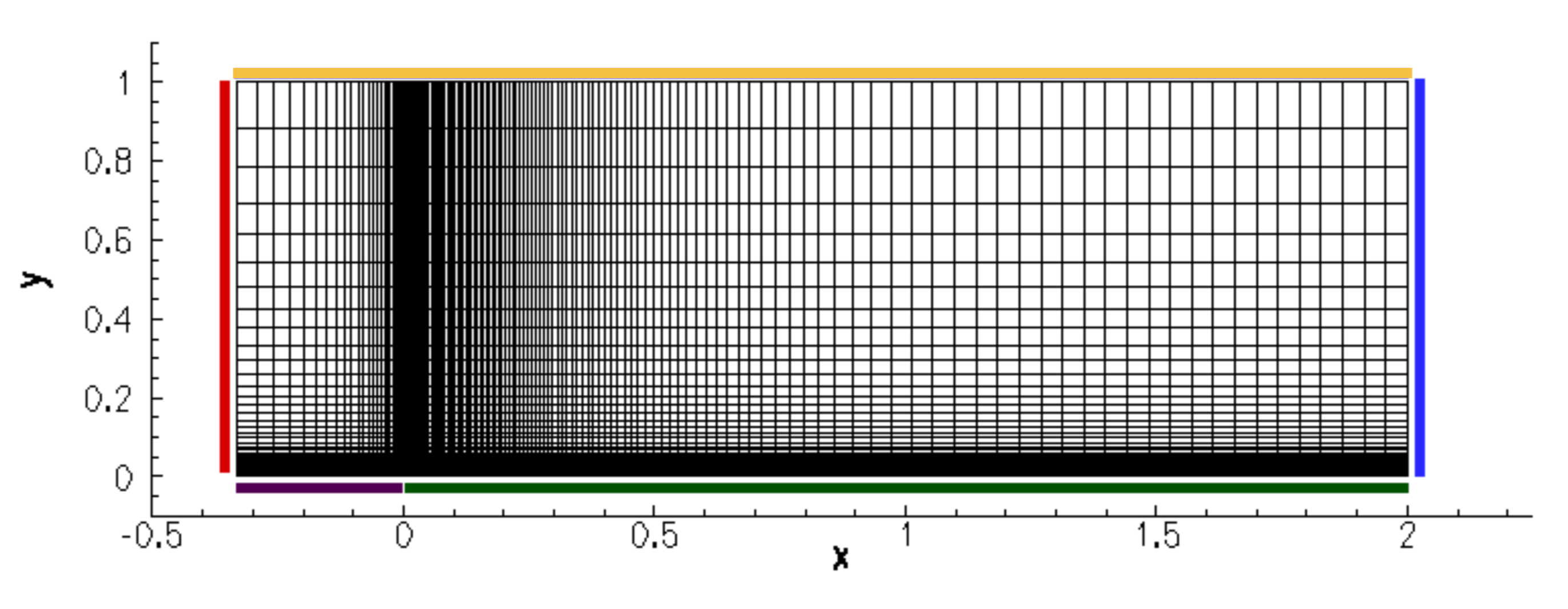 Figure (1): Mesh with boundary conditions: inlet (red), outlet (blue), far-field (orange), symmetry (purple), wall (green).
If you would like to run the flat plate problems for yourself, you can use the files available in the SU2 V&V repository. Configuration files for both the SA and SST cases, as well as all grids in SU2 format, are provided. A Python script is also distributed in order to easily recreate the figures seen below from the data.
Results
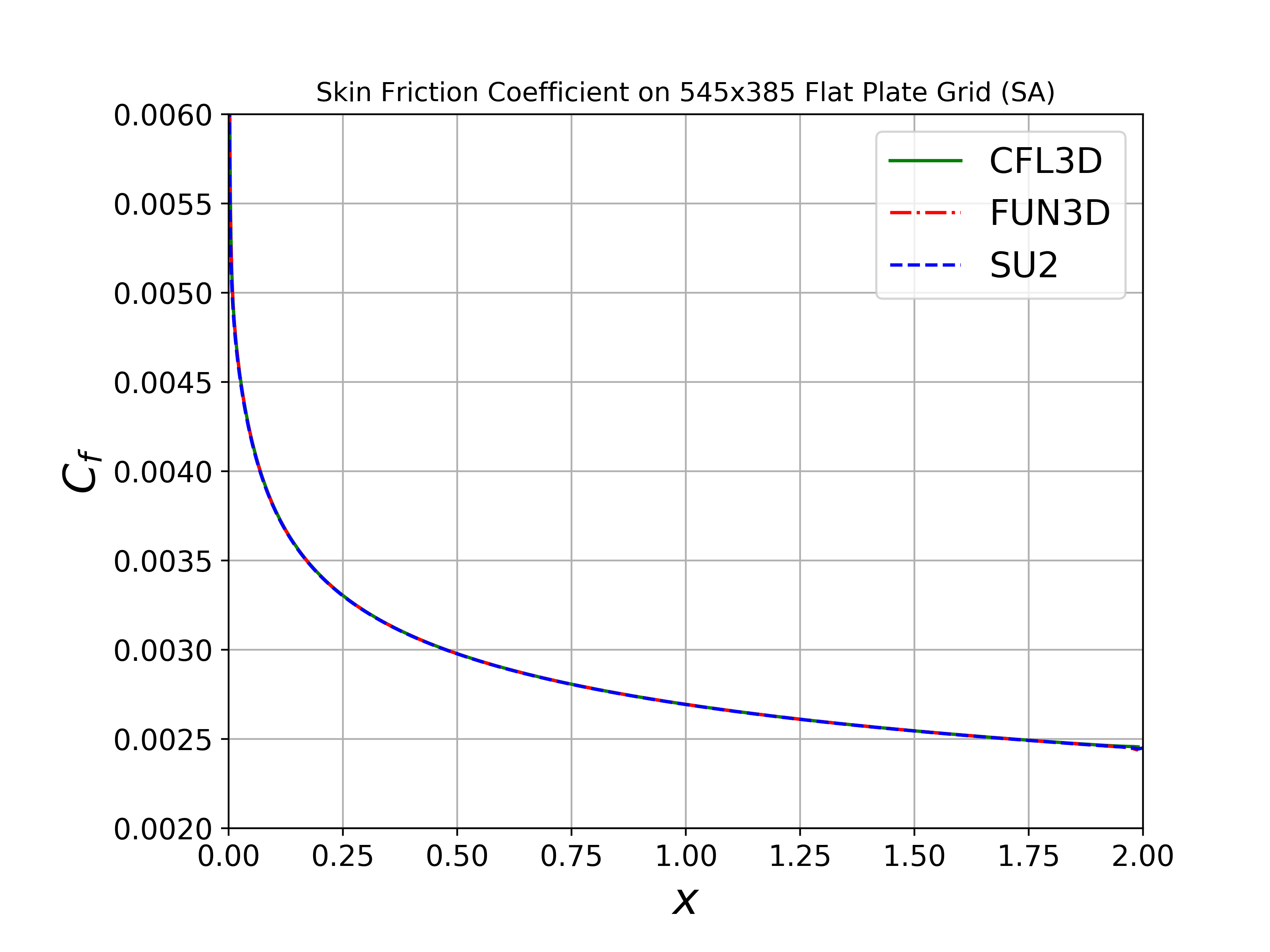
The results for the mesh refinement study are presented and compared to results from FUN3D and CFL3D, including results for both the SA and SST turbulence models.
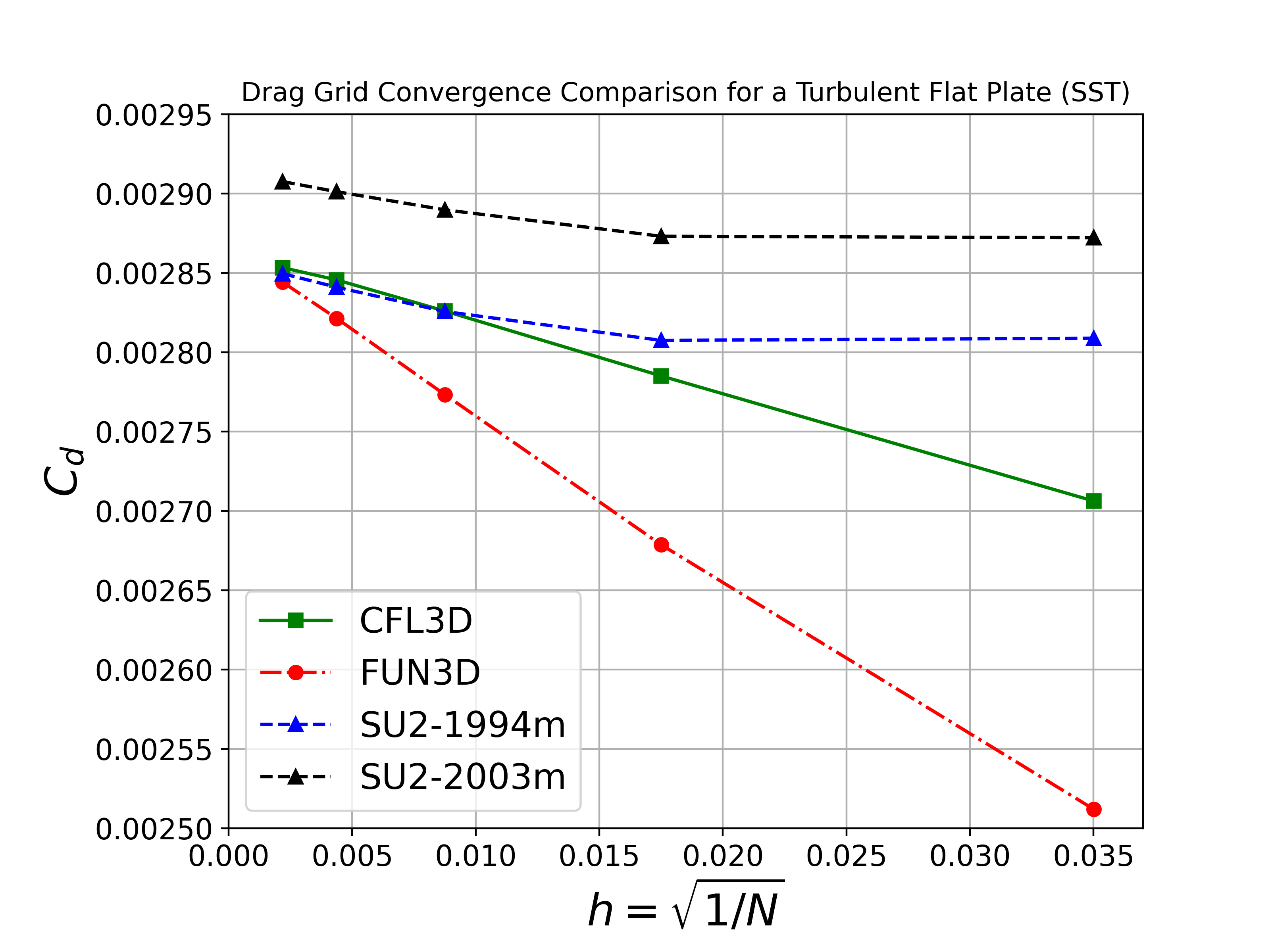
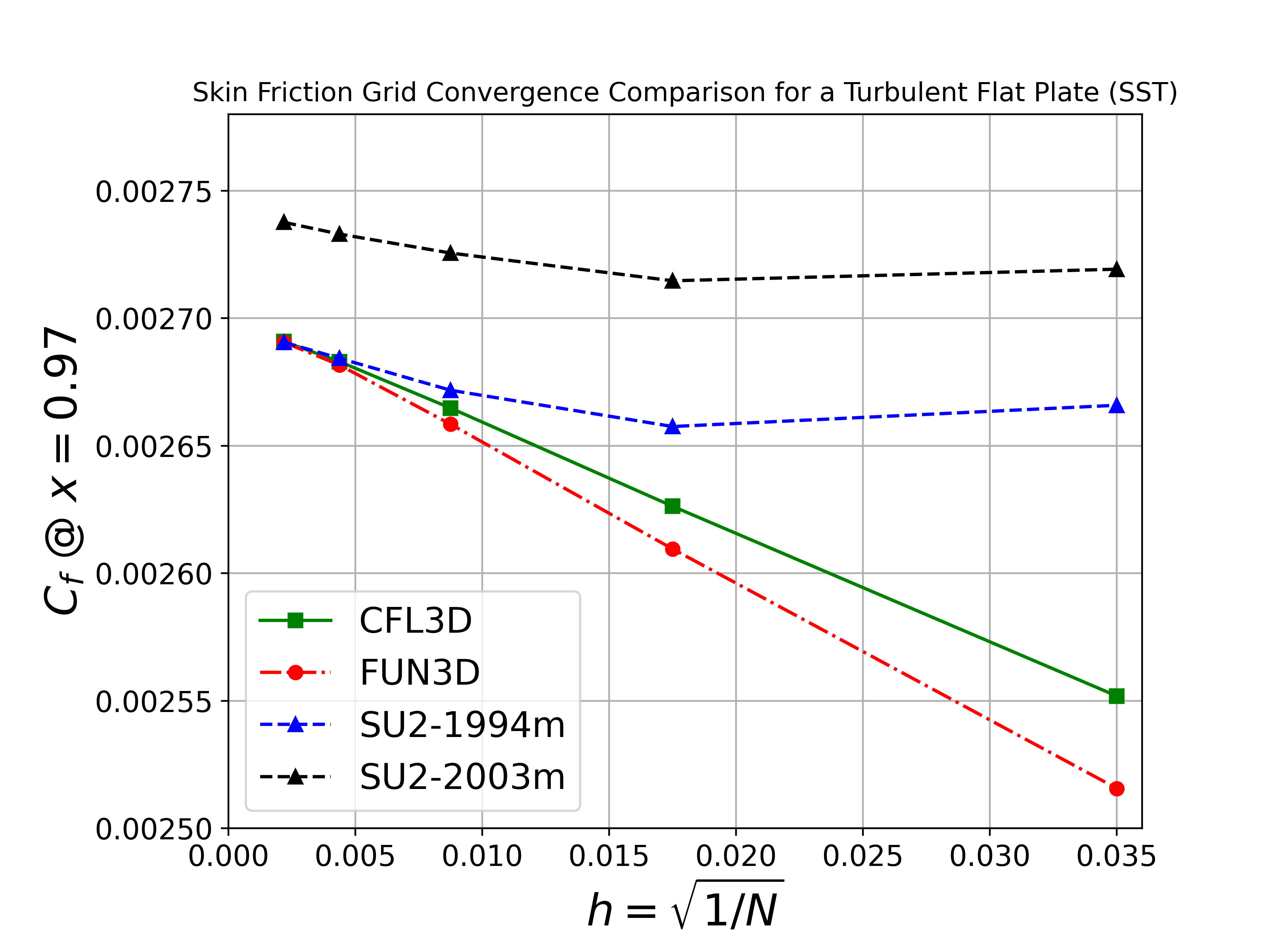
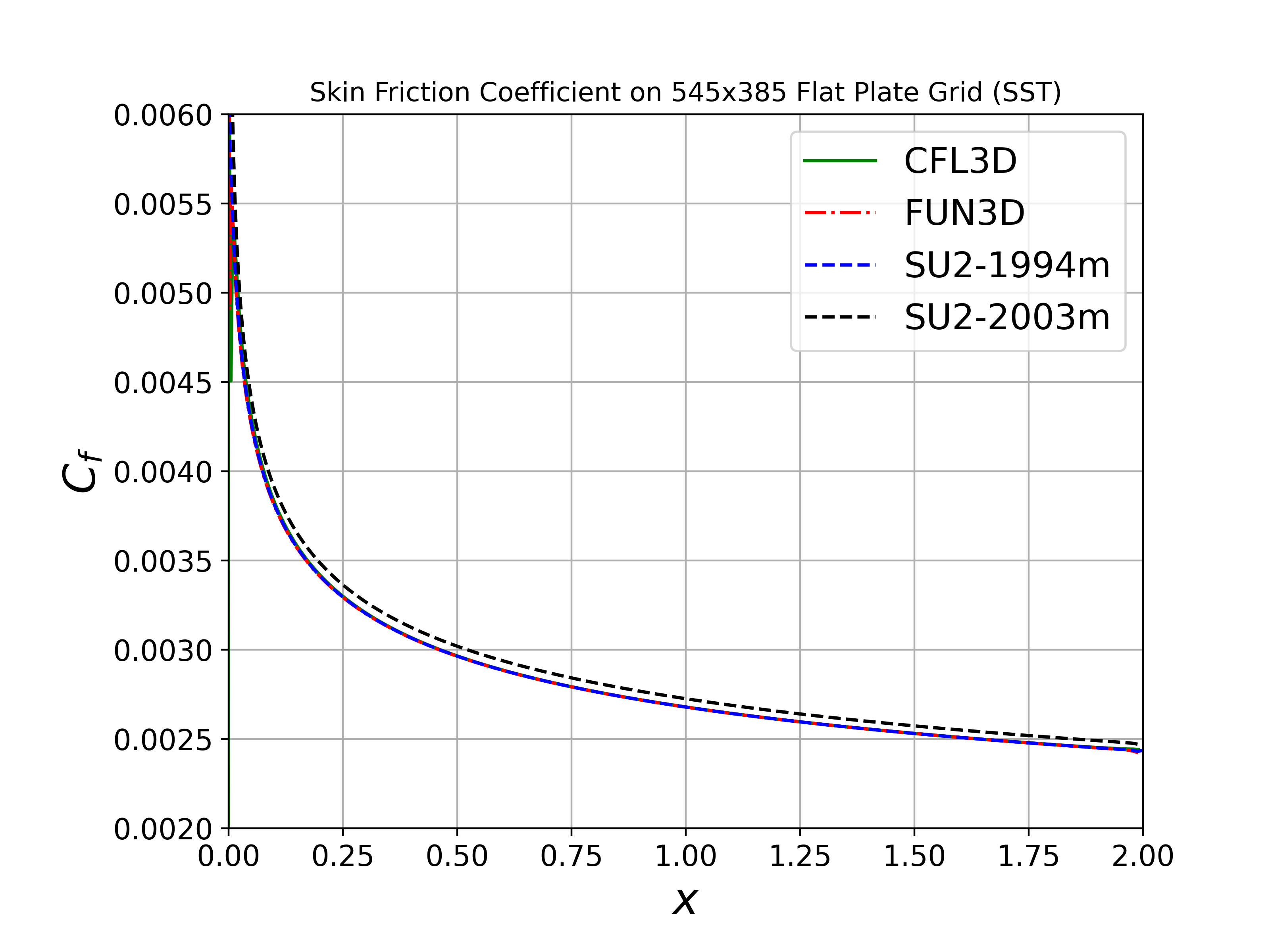
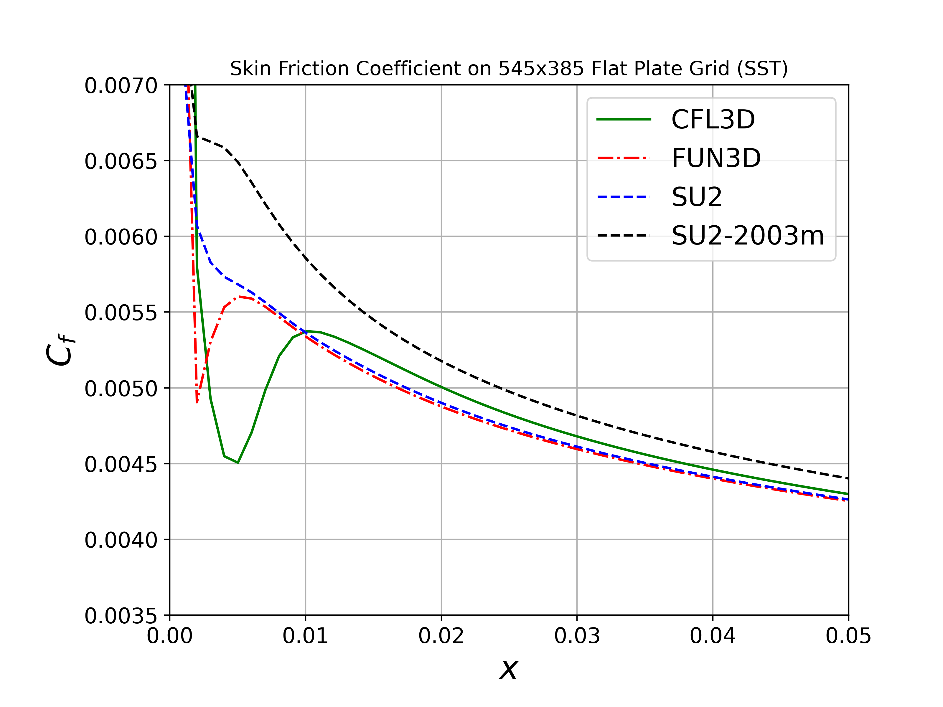
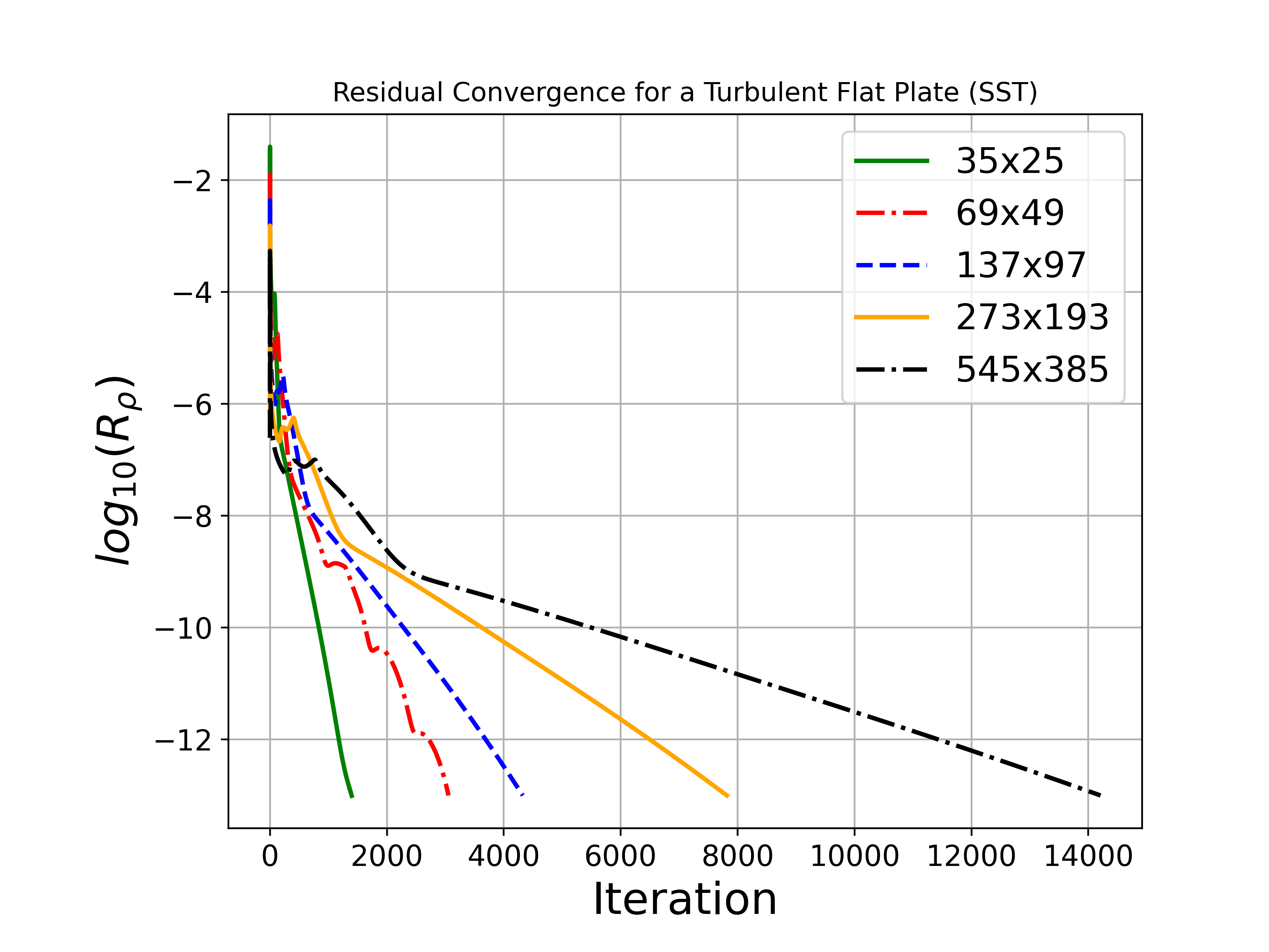
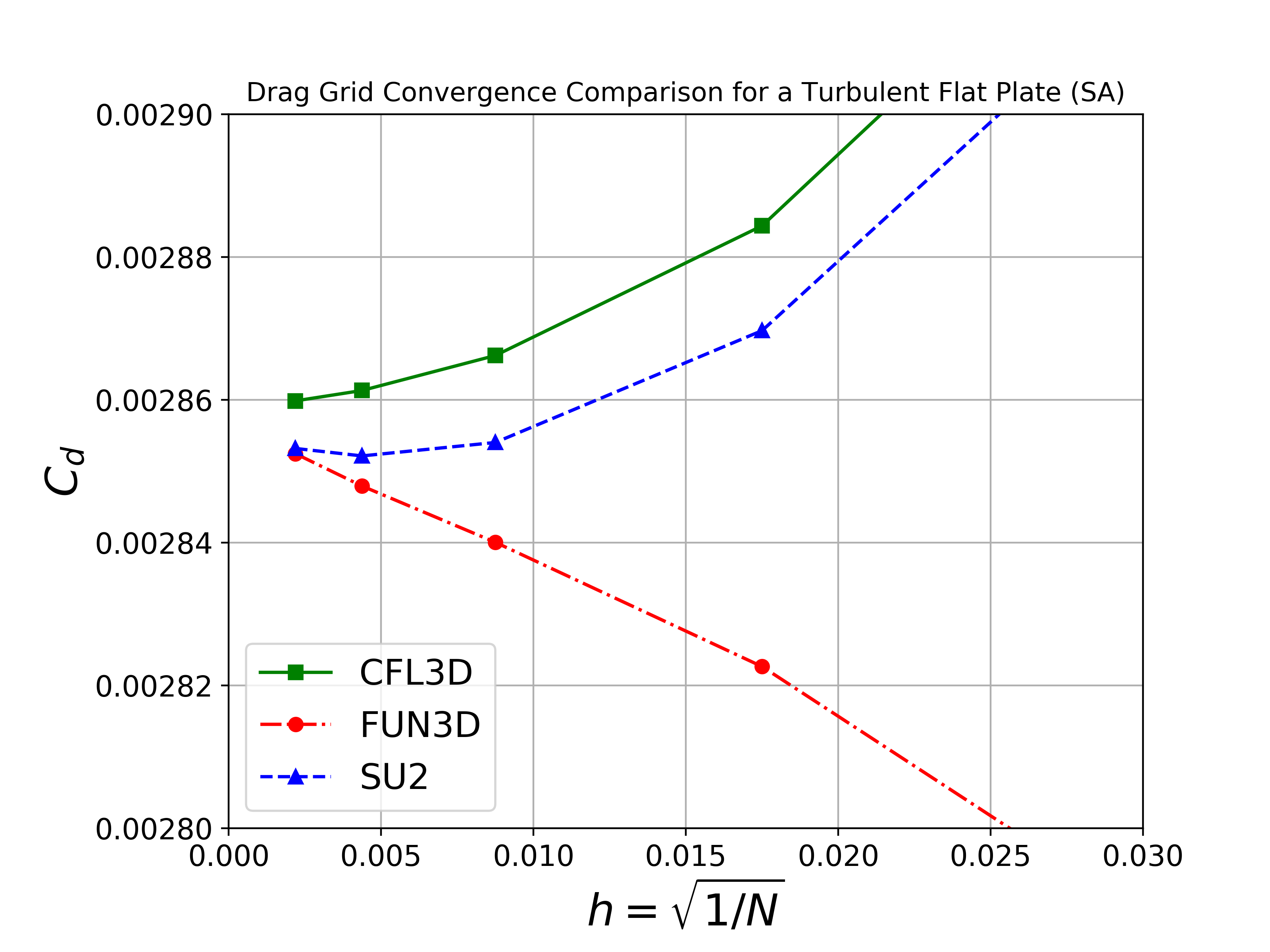
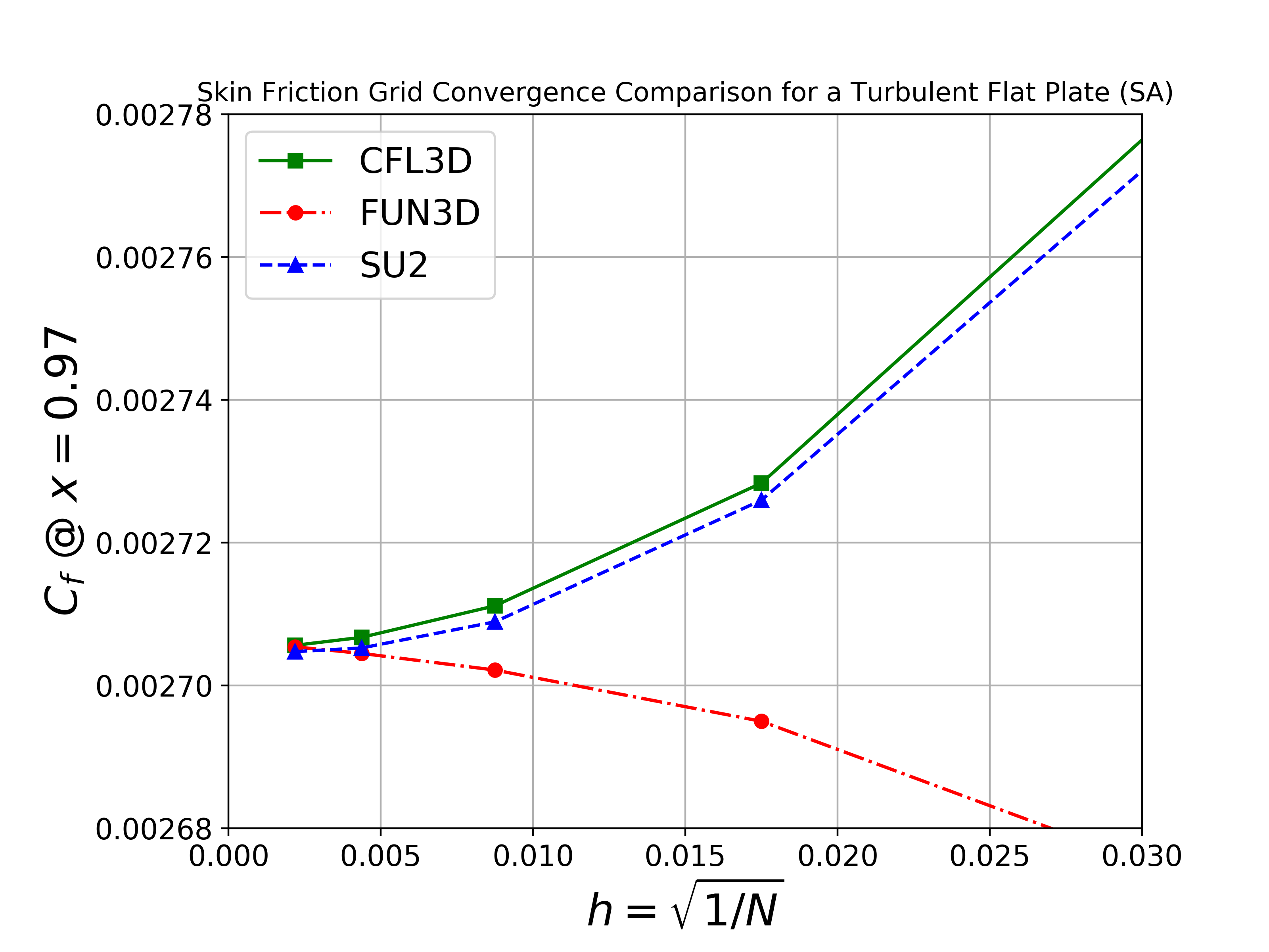
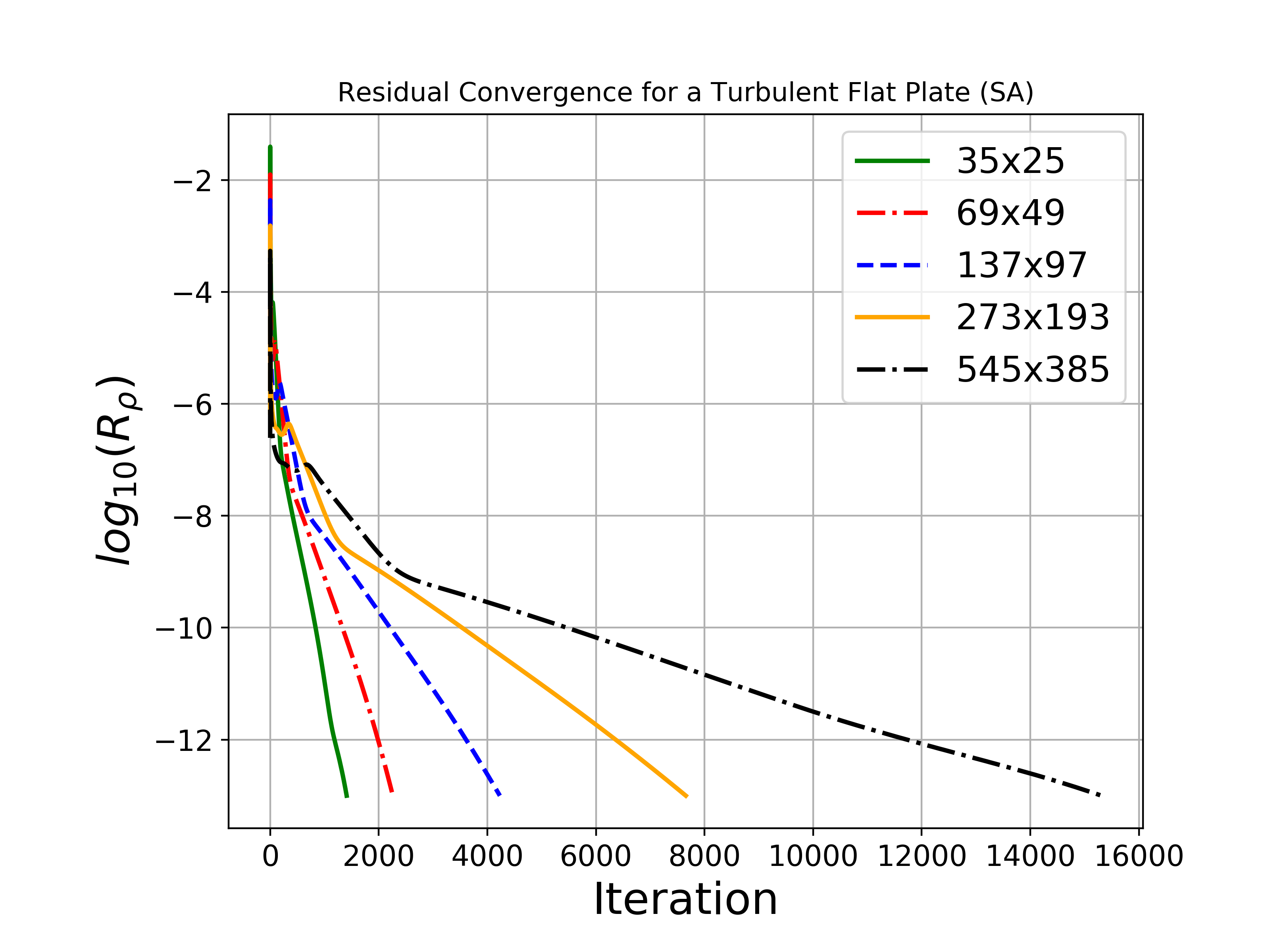
We will compare the convergence of the drag coefficient on the flat plate with grid refinement, as well as the value of the skin friction coefficient at one point on the plate (x = 0.97). We also show the skin friction coefficient plotted along the length of the plate. All cases were converged until the density residual was reduced to 10-13, which is demonstrated by a figure containing residual convergence histories for each mesh.
Both the SA and SST models exhibit excellent agreement in the figures below. With grid refinement, we see that both drag and skin friction values asymptote very close to those of FUN3D and CFL3D (and additional codes not shown here but displayed on the NASA TMR), which builds high confidence in the implementations of these two turbulence models in SU2.
SA Model
SST Model
The two main SST models, 1994m and 2003m, are compared against FUN3D and CFL3D. Note that for FUN3D and CFL3D, for this case only the 1994m results are available.