2D DSMA661 Airfoil Near-Wake RANS Verification Case

The details of the DSMA661 airfoil benchmark validation testcase are taken from the NASA TMR website.

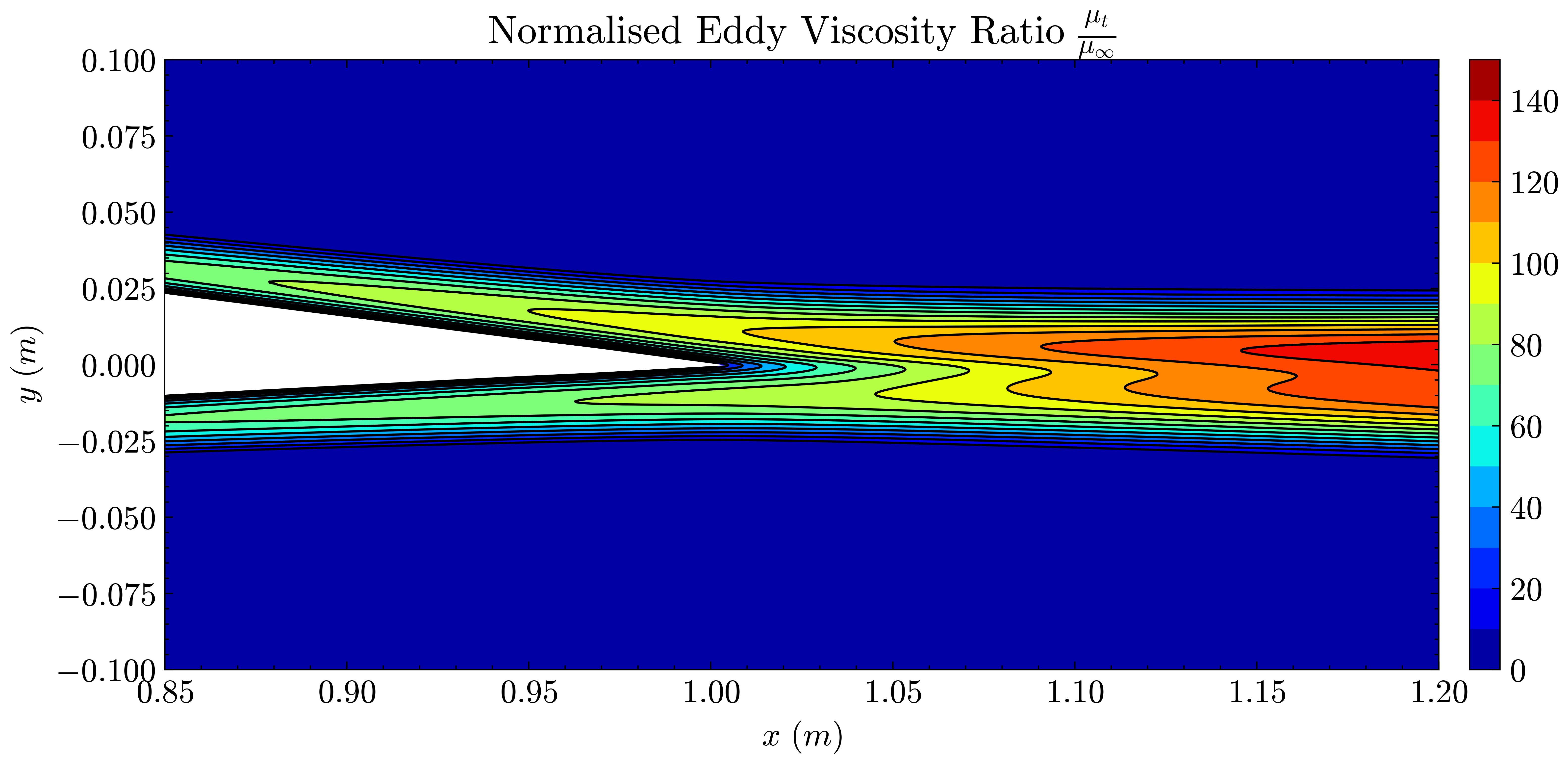
Figure (1): SA model - Normalised Turbulent Viscosity Ratio

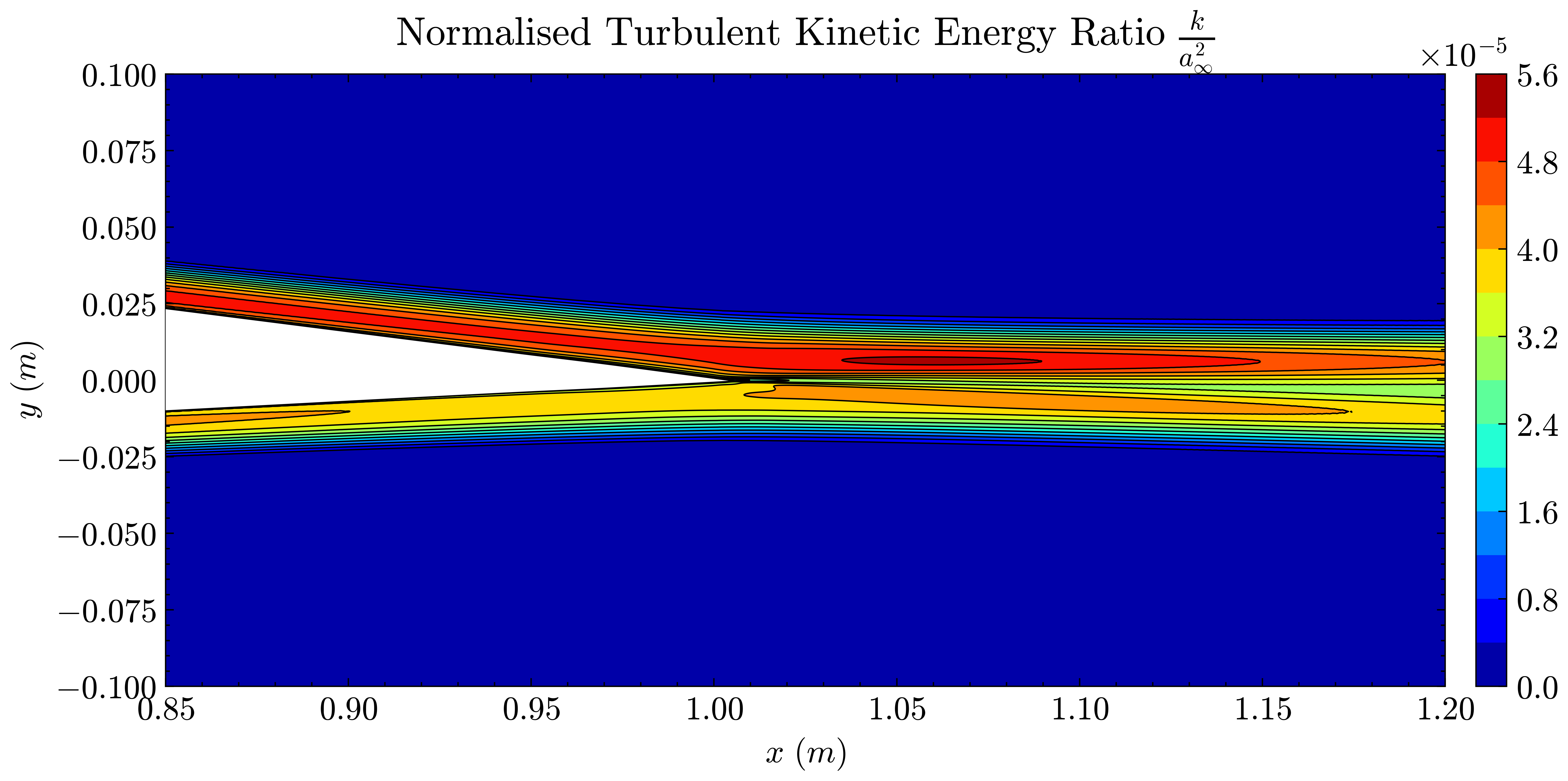
Figure (2): SST model - Normalised Turbulent Kinetic Energy Ratio

By comparing the SU2 given results of the DSMA661 testcase against the CFL3D and FUN3D codes on a sequence of refined grids, an agreement of aerodynamic quantities builds a high degree of confidence that the implemented SA and SST turbulence models are correct. Therefore the goal of this case is to verify the implementations of the SA and SST models in SU2.

Problem Setup

The DSMA661 case is a low Mach (incompressible) test case, used to verify implementations of compressible sovlers. A C-grid domain is used whose schematic is shown in the figure below:

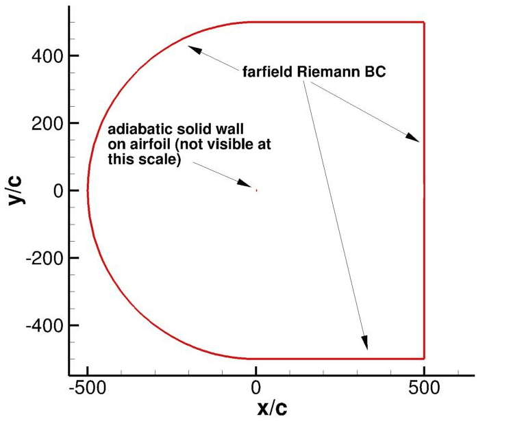Figure (3): Computational domain of the Testcase

The farfield is defined as a Reimann boundary condition with a fully turbulent inflow condition prescribed. The airfoil has sharp trailing edge with a chord length of 1m, represented by an adiabatic no-slip wall boundary condition.

This problem will solve the flow past the airfoil with the following flow properties:

• Freestream Temperature = 300 K
• Freestream Mach number = 0.088
• Reynolds Number = 1.2E6
• Ref. Reynolds Length (chord) = 1.0 m
• Viscosity Model = Sutherland
• Angle of Attack = 0°

Mesh Description

Structured meshes increasing in density are used to perform the grid independence study. The meshes are taken from the NASA TMR website, converted from the CGNS format to SU2’s ASCII mesh format. Each grid is split into two zones; one covering the airfoil and another extending into the wake region. The figure below shows a schematic of the domain parametrisation.

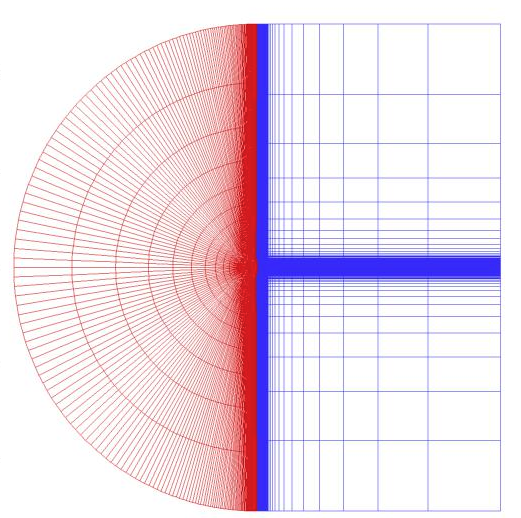Figure (4): Example depiction of the discretised mesh

The airfoil surface is represented by 65 points on the coarsest mesh and 1025 on the finest. The meshes are named according to the number of nodes in the x and y directions, respectively, as follows:

1. 149x25 - 4144 Quadrilaterals
2. 297x57 - 16576 Quadrilaterals
3. 513x113 - 66304 Quadrilaterals
4. 1185x225 - 265216 Quadrilaterals
5. 2369x449 - 1060864 Quadrilaterals

If you would like to run the DSMA661 testcase problem for yourself, the files used in this study are available in the SU2 V&V repository. This includes the configuration files for both SA and SST cases as well as the grids in SU2 format.

Results

The results for the mesh refinement study are presented and compared to results from FUN3D and CFL3D, including results for both SA and SST turbulence models.

To keep the comparisons consistent with these solvers, the results shown use the standard SA model and V2003m SST turbulence models. For SA model, the turbulent inflow is defined by $\tilde{\nu} = 3 \nu_{\infty}$ and $k/w$=0.009 for SST. The ROE scheme (with kappa=0.33333) is used with MUSCL treatment on the convective terms with a VAN ALBADA EDGE limiter and first order treatment on the turbulent advective terms. All cases were converged until the density residual was reduced to 10^-11. More details about the FUN3D and CFL3D set ups can found on the NASA TMR website.

We will compare the convergence of lift and drag force values, splitting the drag into its pressure and viscous terms, and the minimum x-velocity in the wake regions at certain points. The coefficients of pressure and skin friction over the airfoil surface, velocity profiles in the wake region and the eddy viscosity contours will also be compared.

Both the SA and SST models exhibit excellent agreement in the figures below. With grid refinement, we see that the asymptotic force values and minimum velocity values in the wake region reach very close to those of the FUN3D and CFL3D. The differences between the experimental and numerical results arise from the use of a blunt trailing edge in the experiments and a sharp one in the simulations. Nonetheless the CFD codes demonstrate a high degree of accuracy.

Additional codes have been compared against the FUN3D and CFL3D results, and are available on the NASA TMR website. Overall this builds a high degree of confidence in the implementations of these turbulence models in SU2.

SA Model

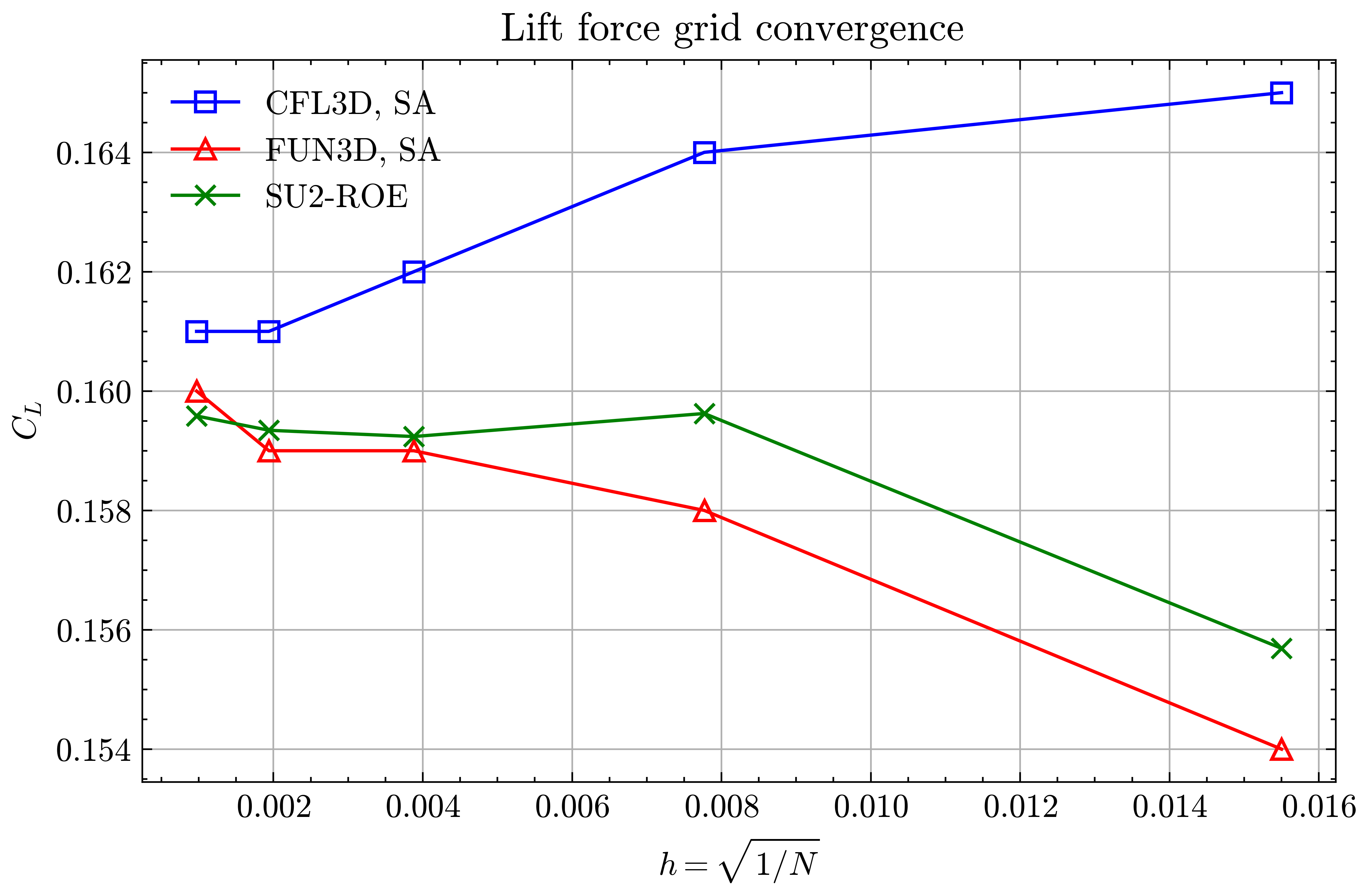
Figure (5): Lift force grid convergence

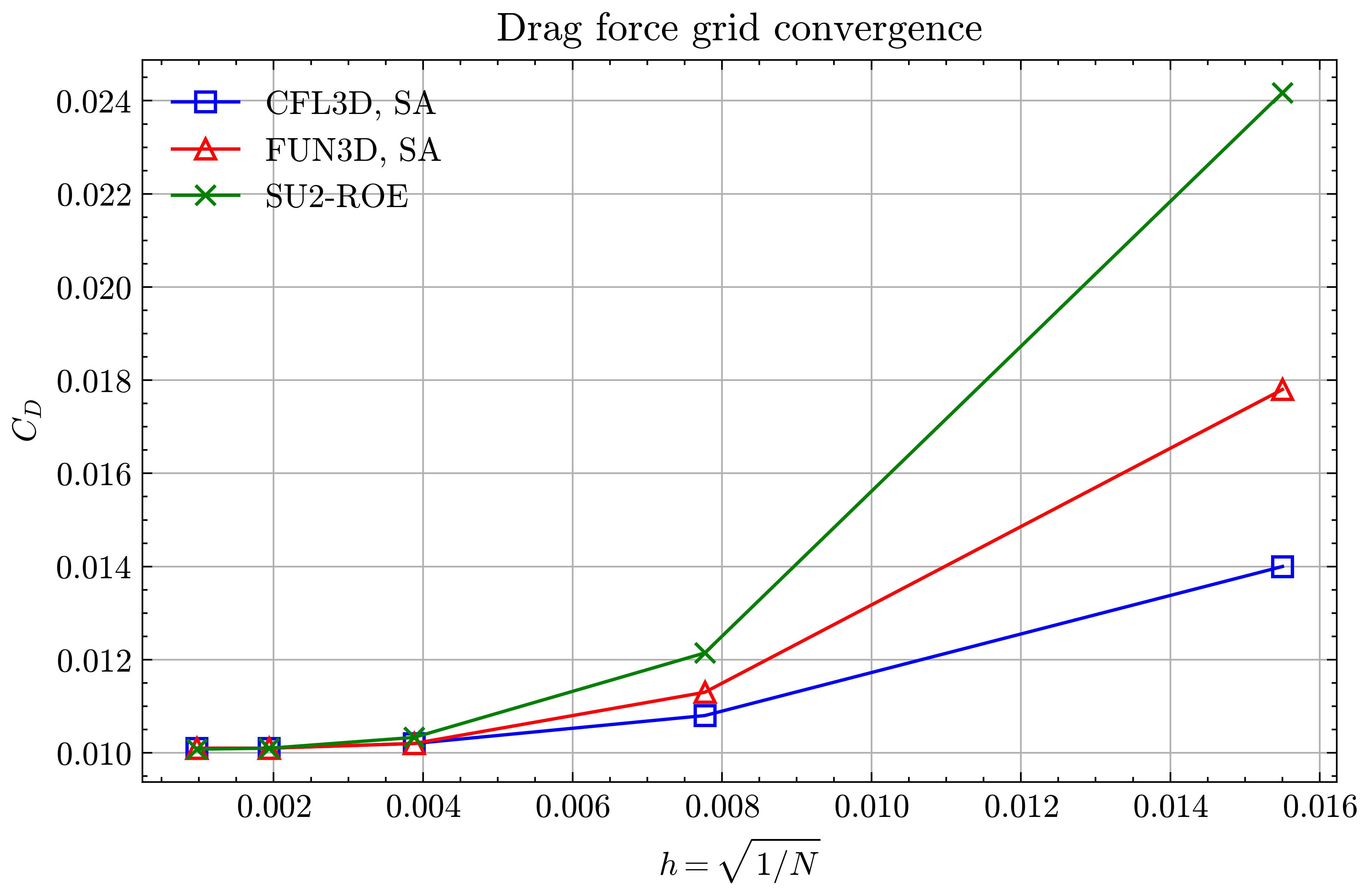
Figure (6): Drag force grid convergence

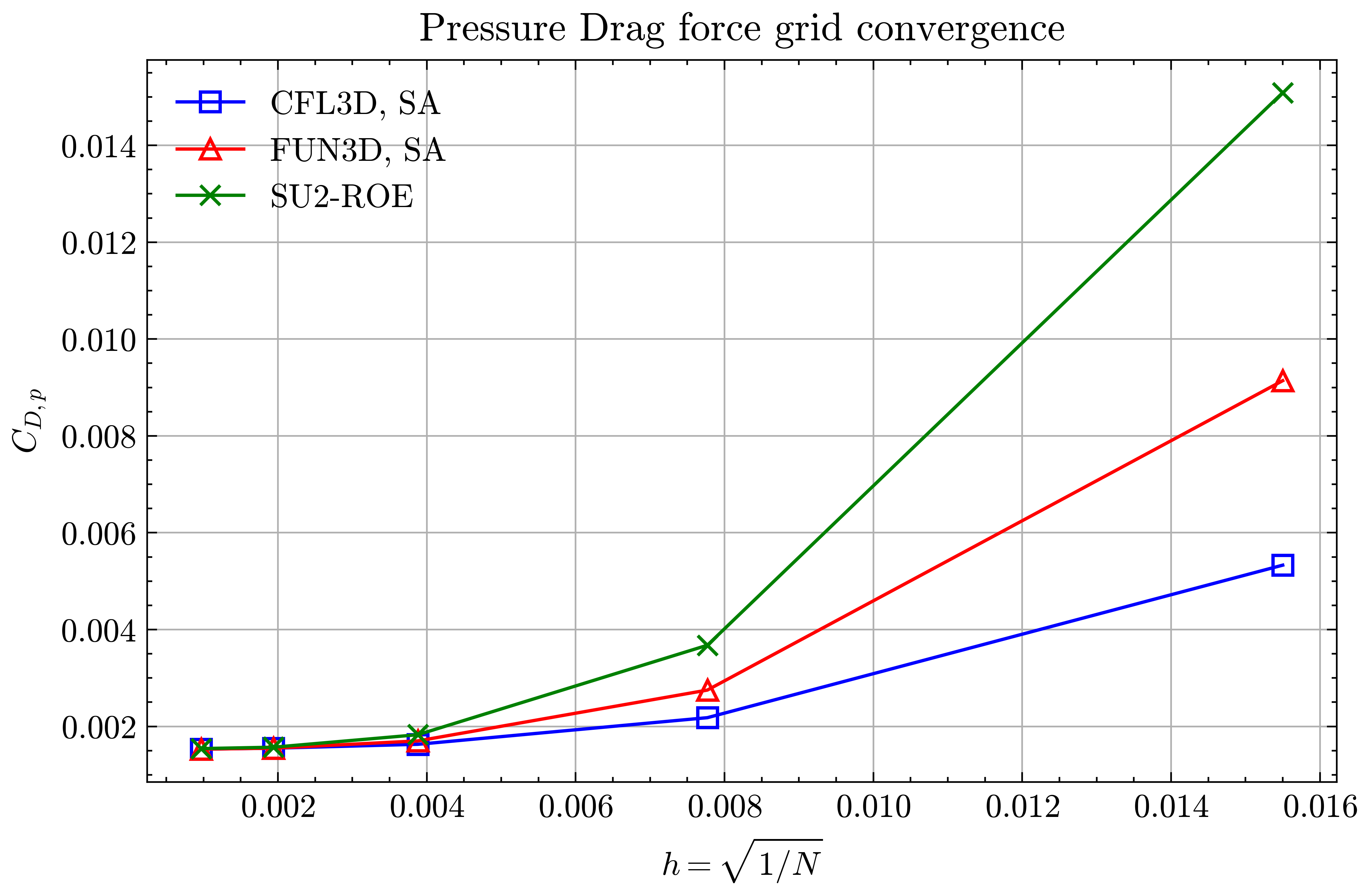
Figure (7): Pressure Drag force grid convergence

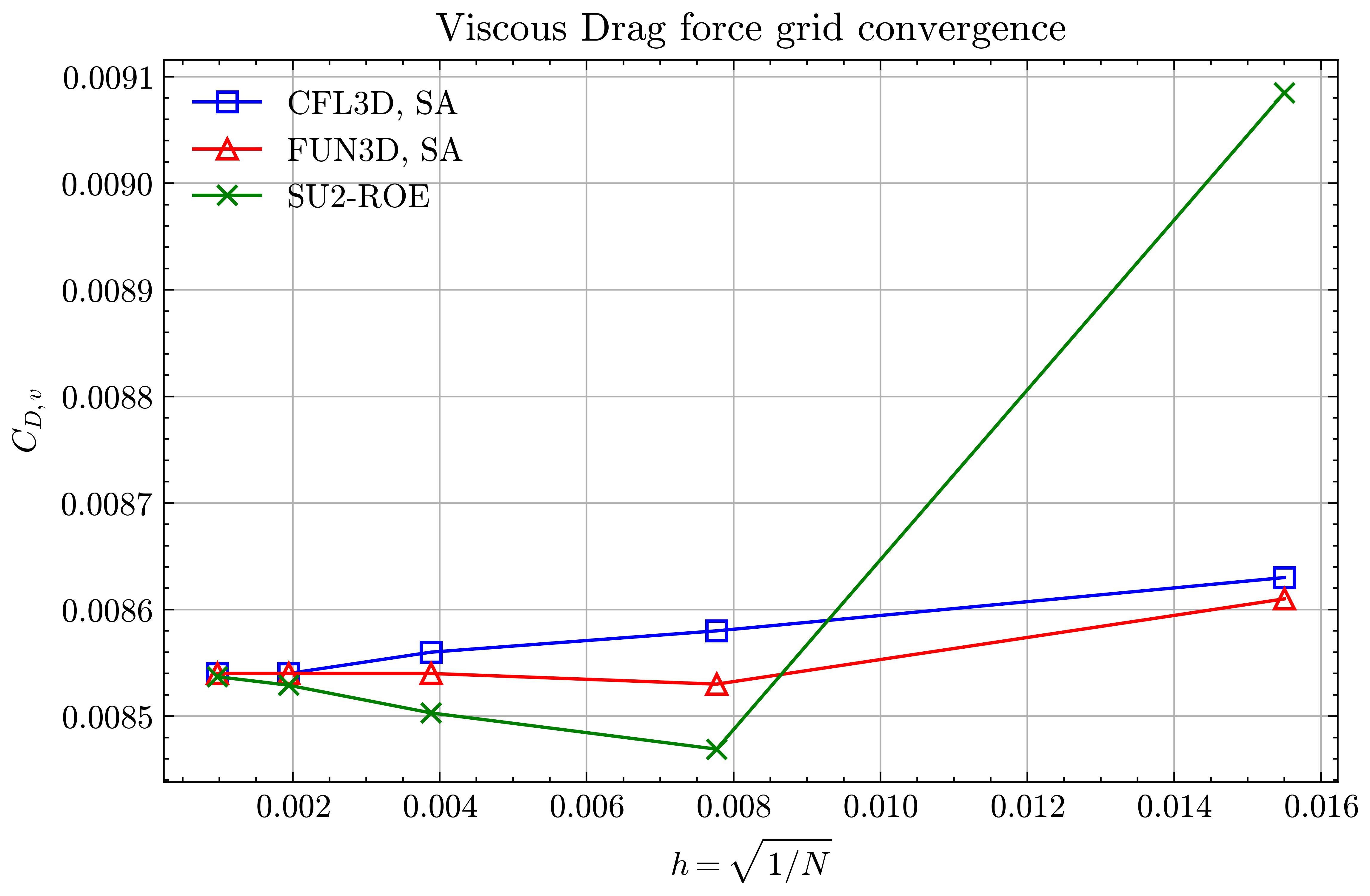
Figure (8): Viscous Drag force grid convergence

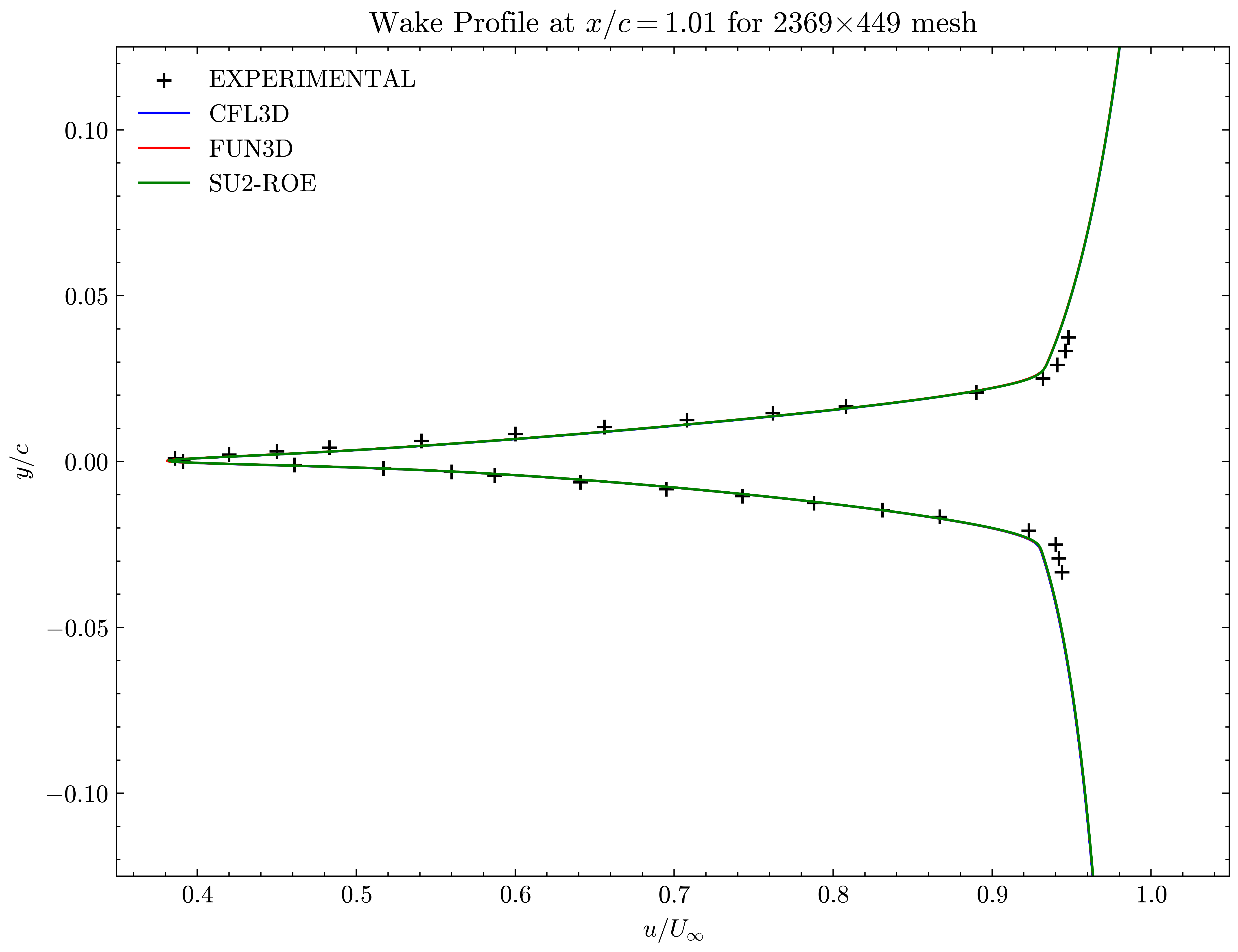
Figure (9): Wake profile at x/c=1.01

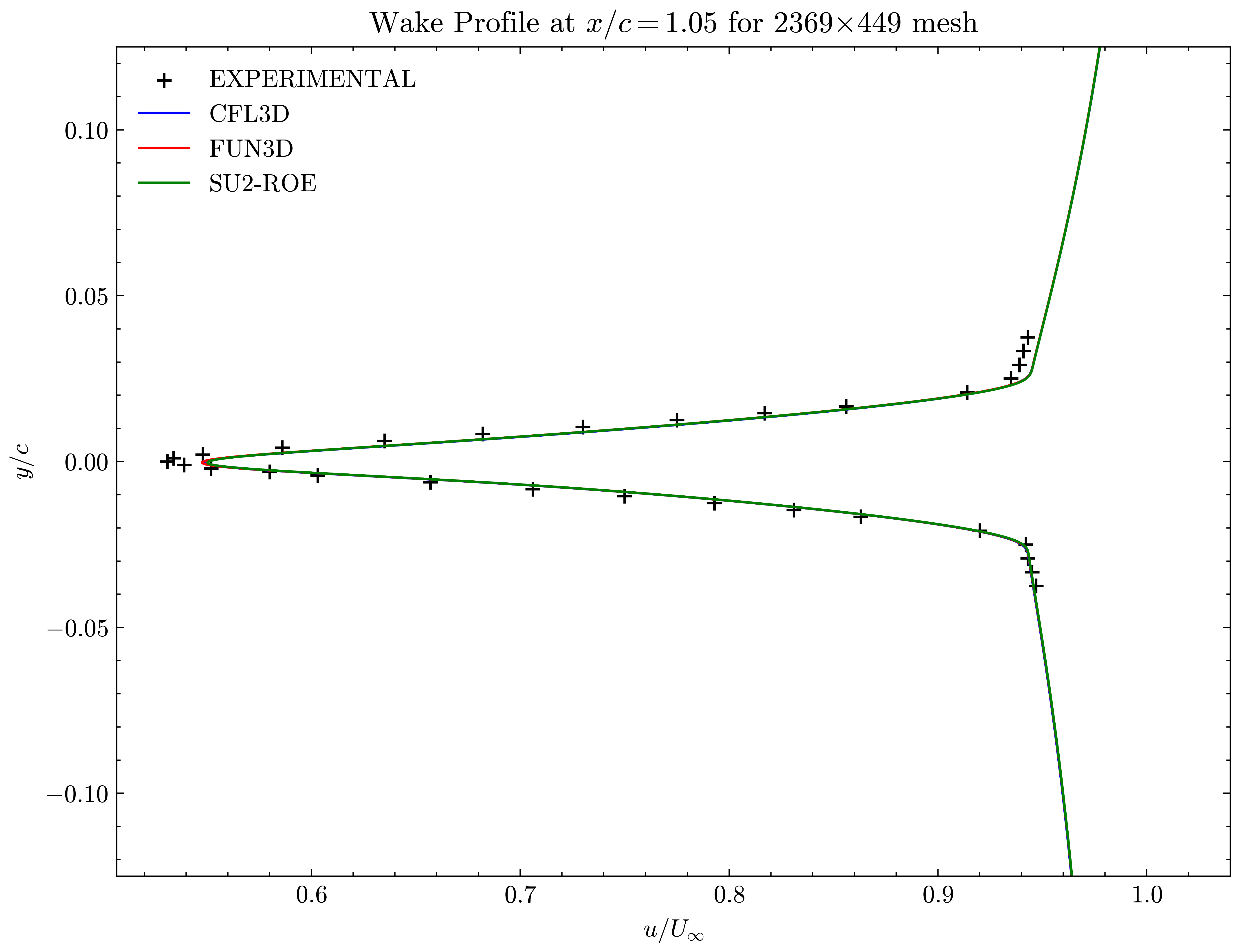
Figure (10): Wake profile at x/c=1.05

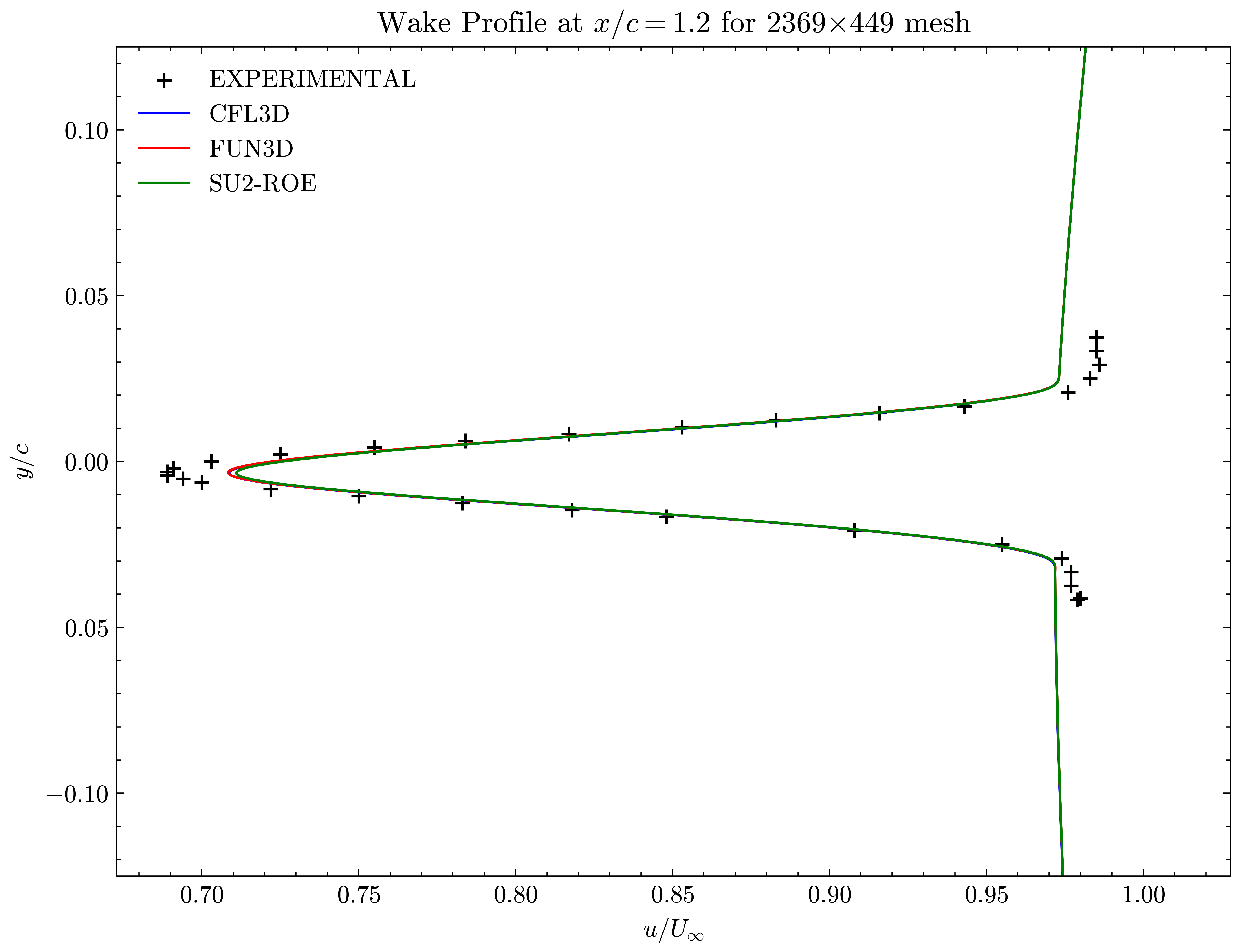
Figure (11): Wake profile at x/c=1.20

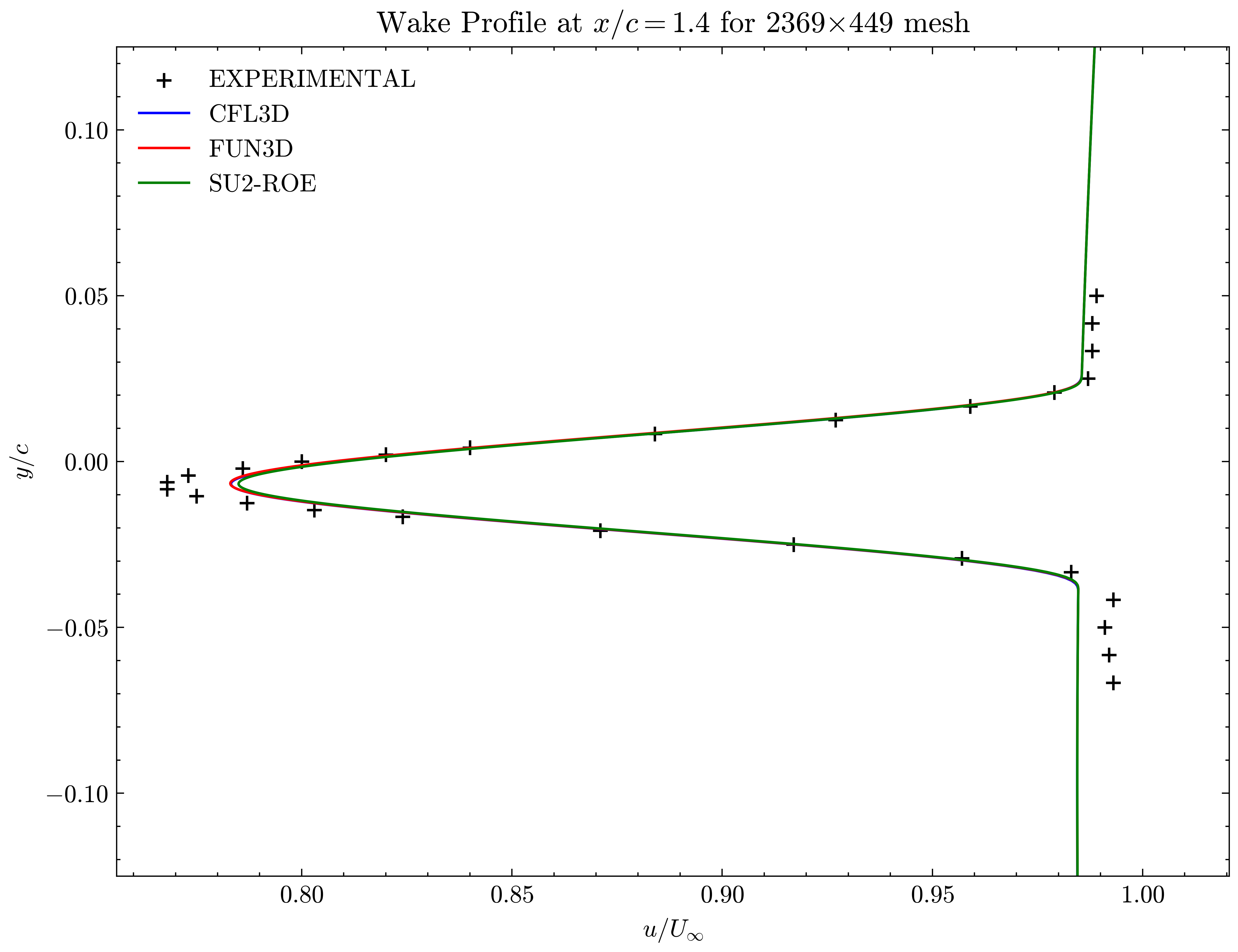
Figure (12): Wake profile at x/c=1.40

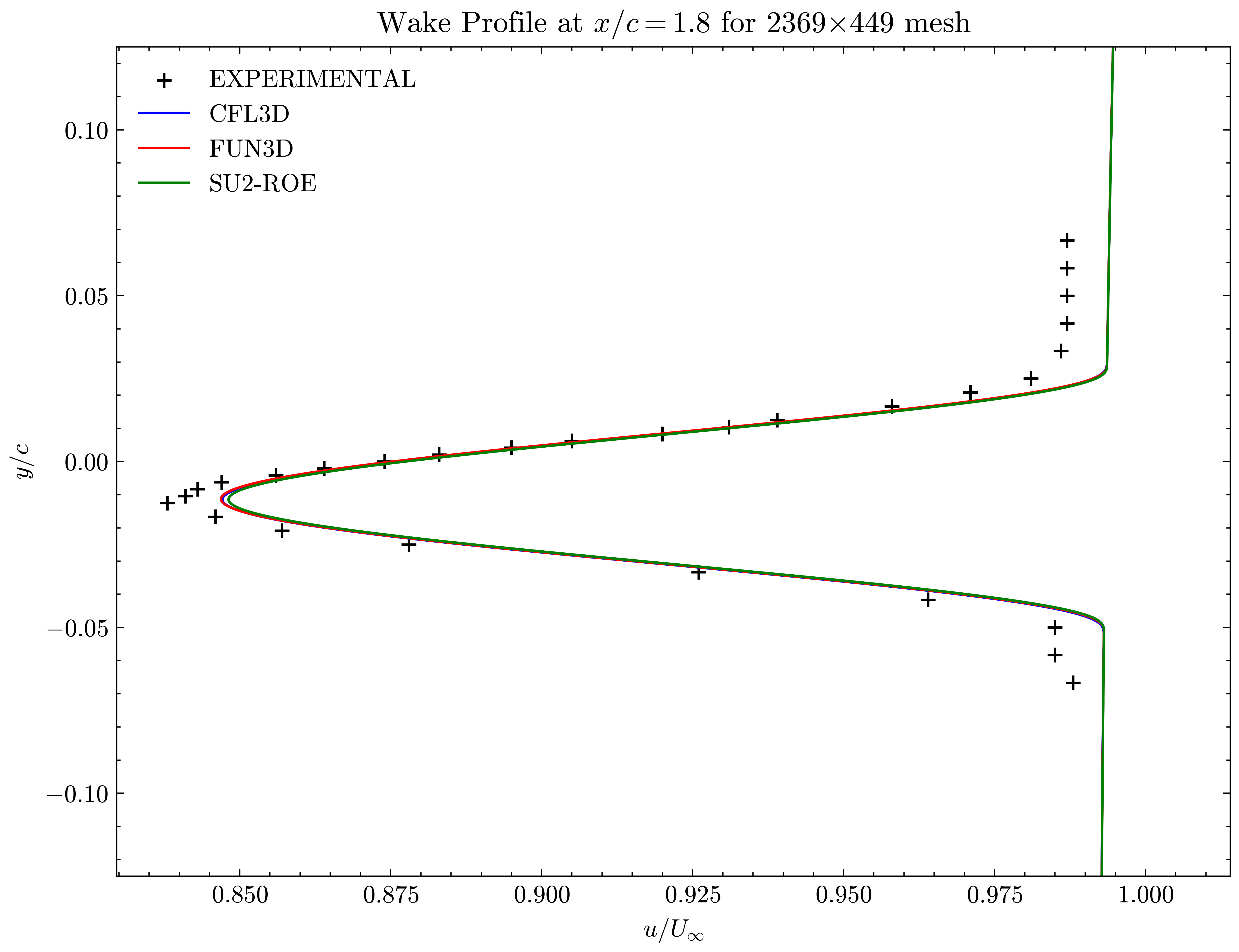
Figure (13): Wake profile at x/c=1.80

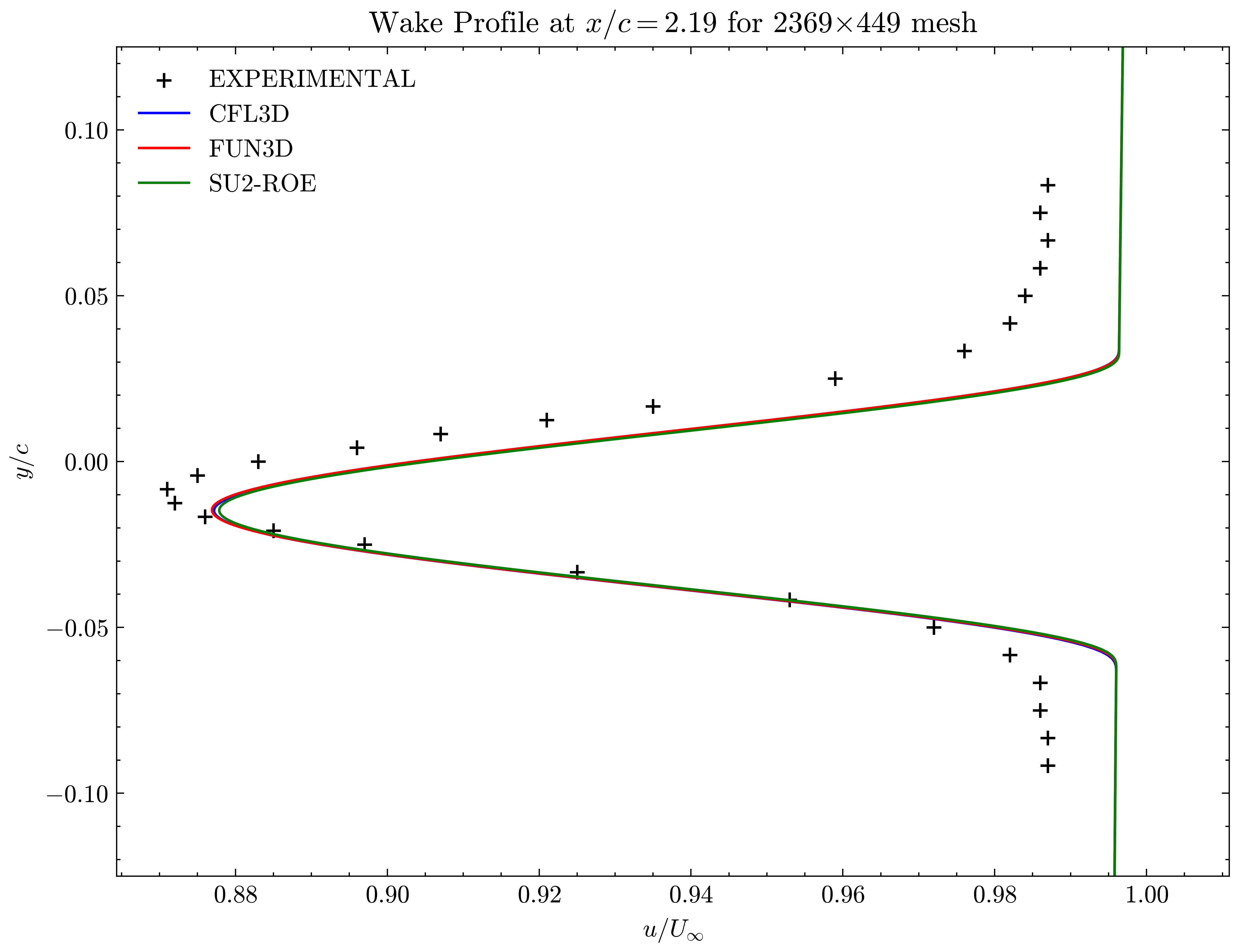
Figure (14): Wake profile at x/c=2.19

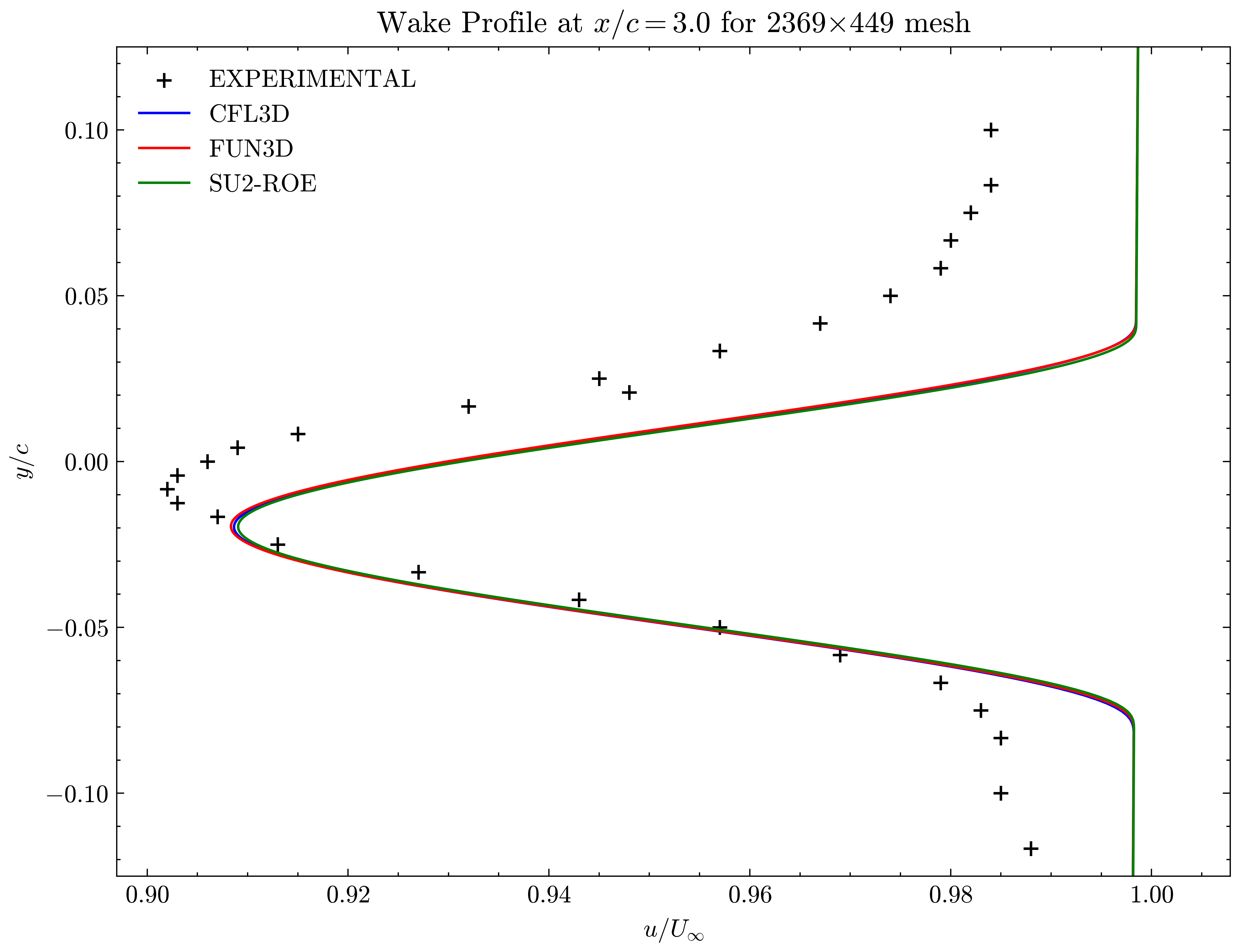
Figure (15): Wake profile at x/c=3.00

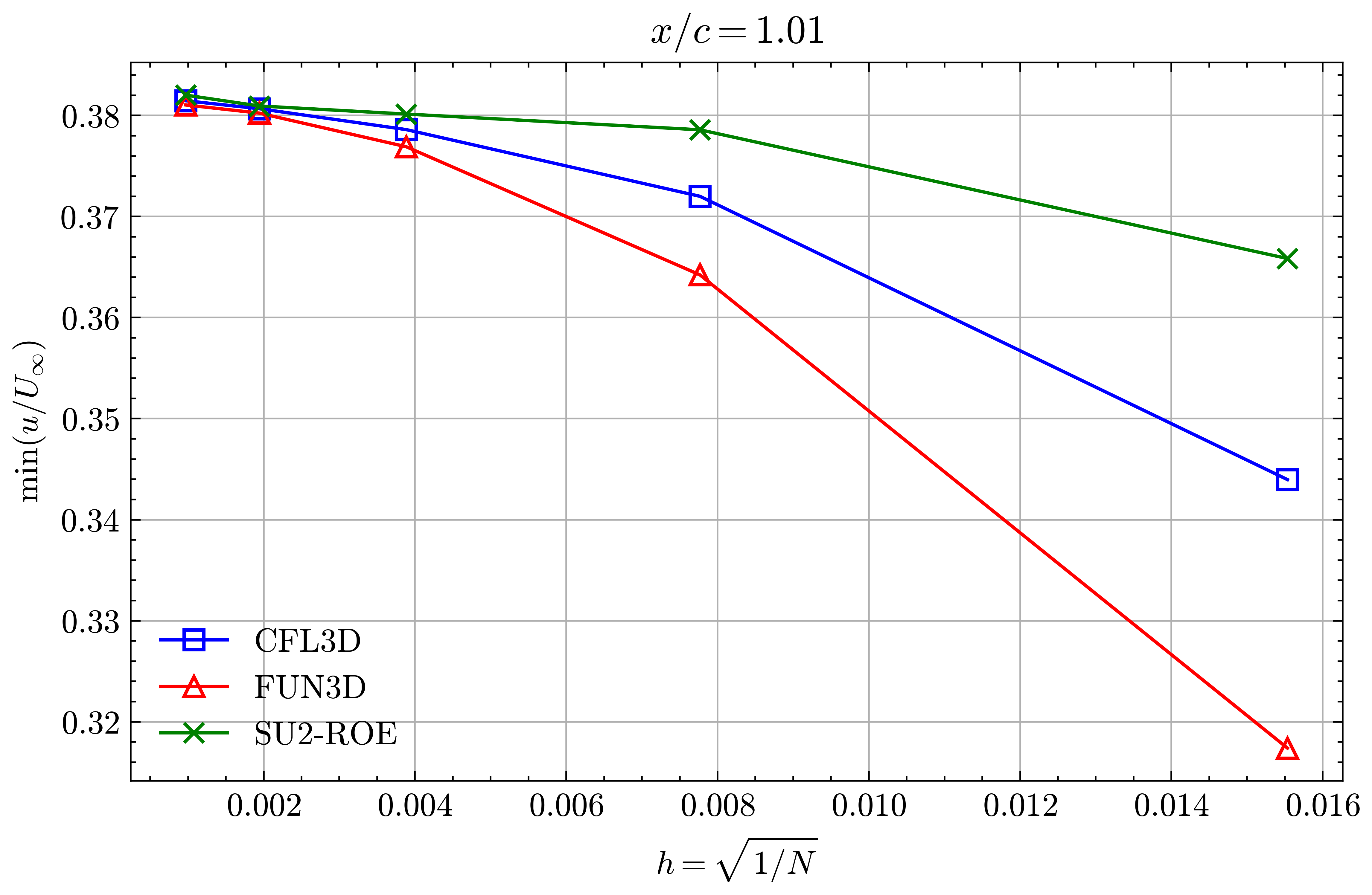
Figure (16): Min x-velocity in Wake profile grid convergence at x/c=1.01

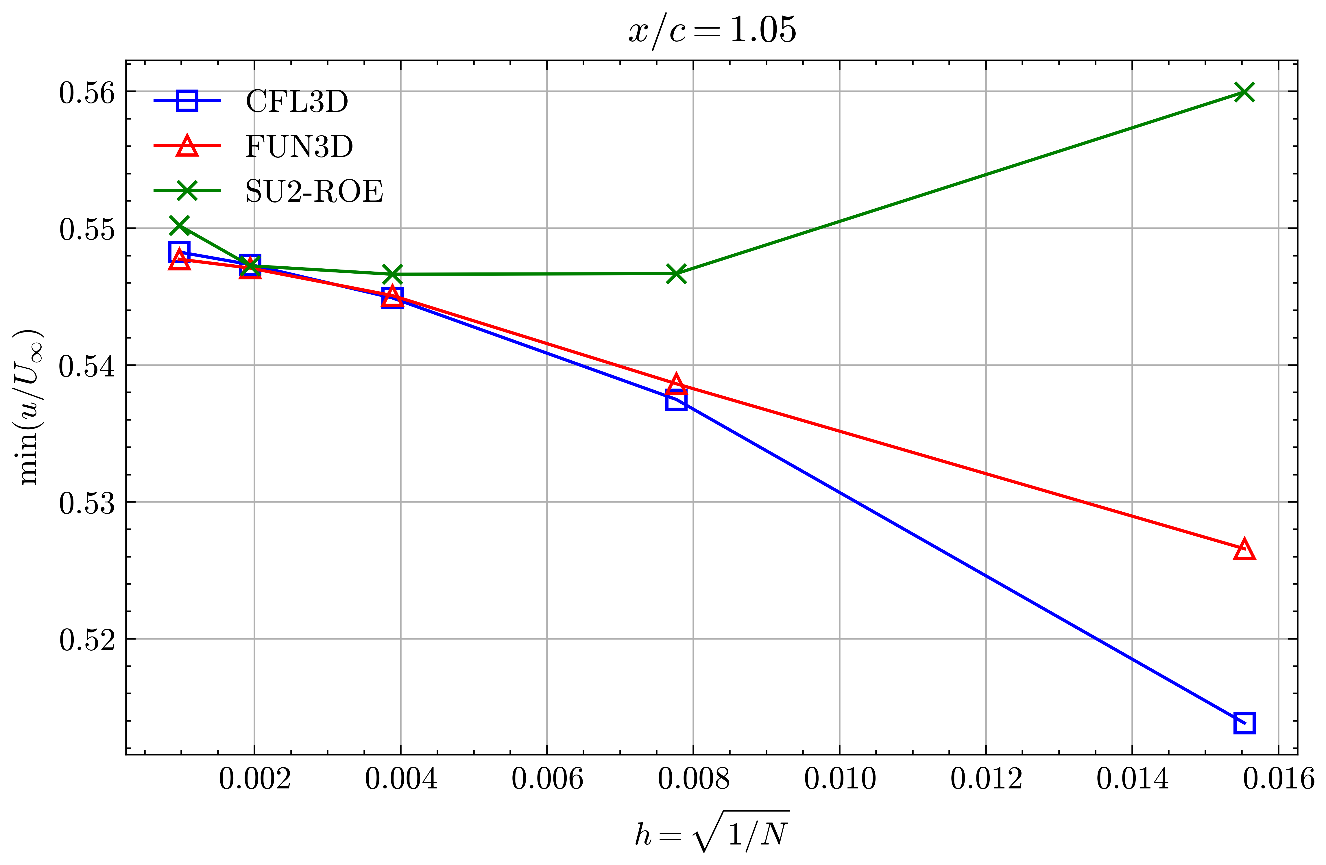
Figure (17): Min x-velocity in Wake profile grid convergence at x/c=1.05

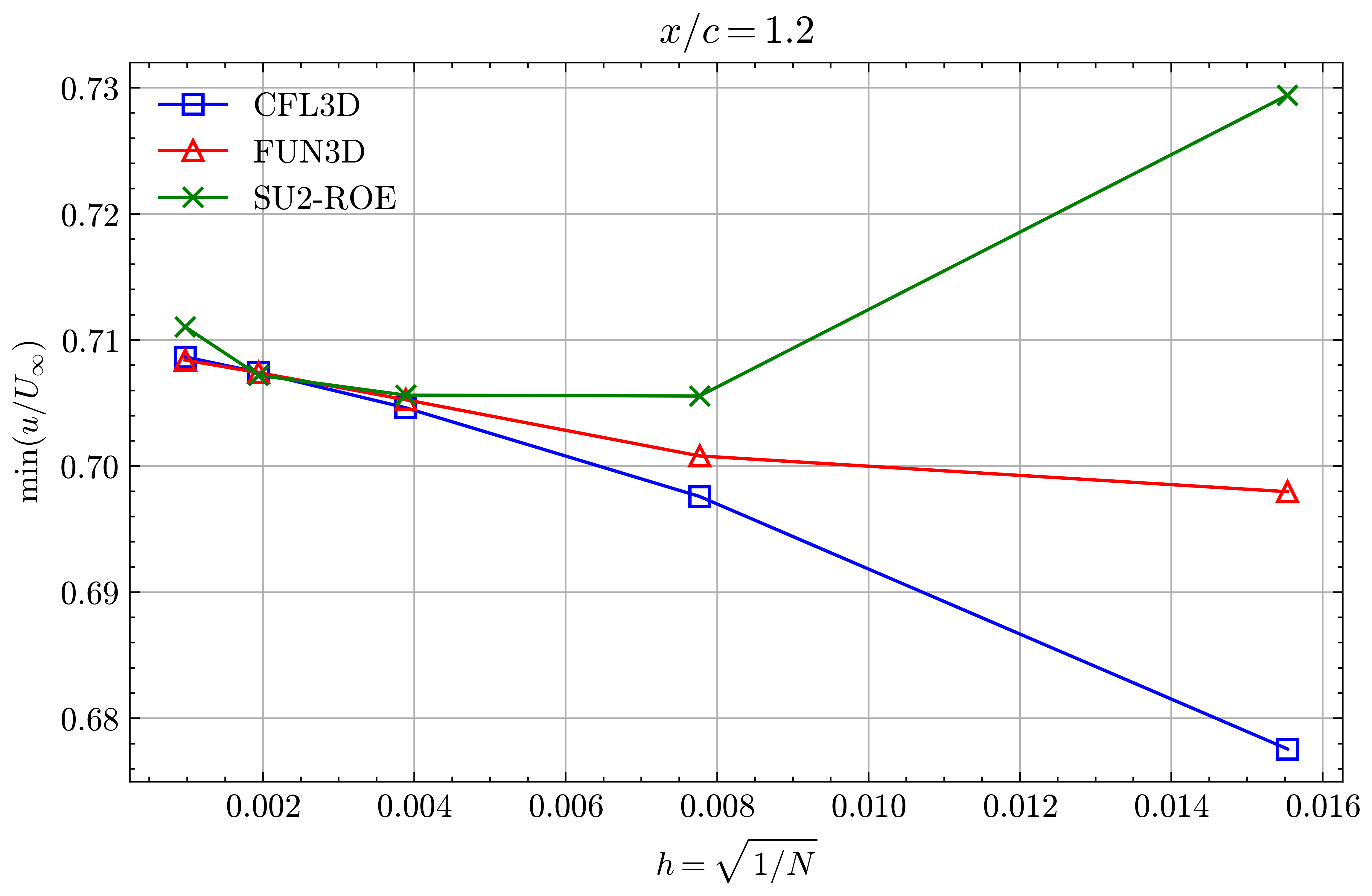
Figure (18): Min x-velocity in Wake profile grid convergence at x/c=1.20

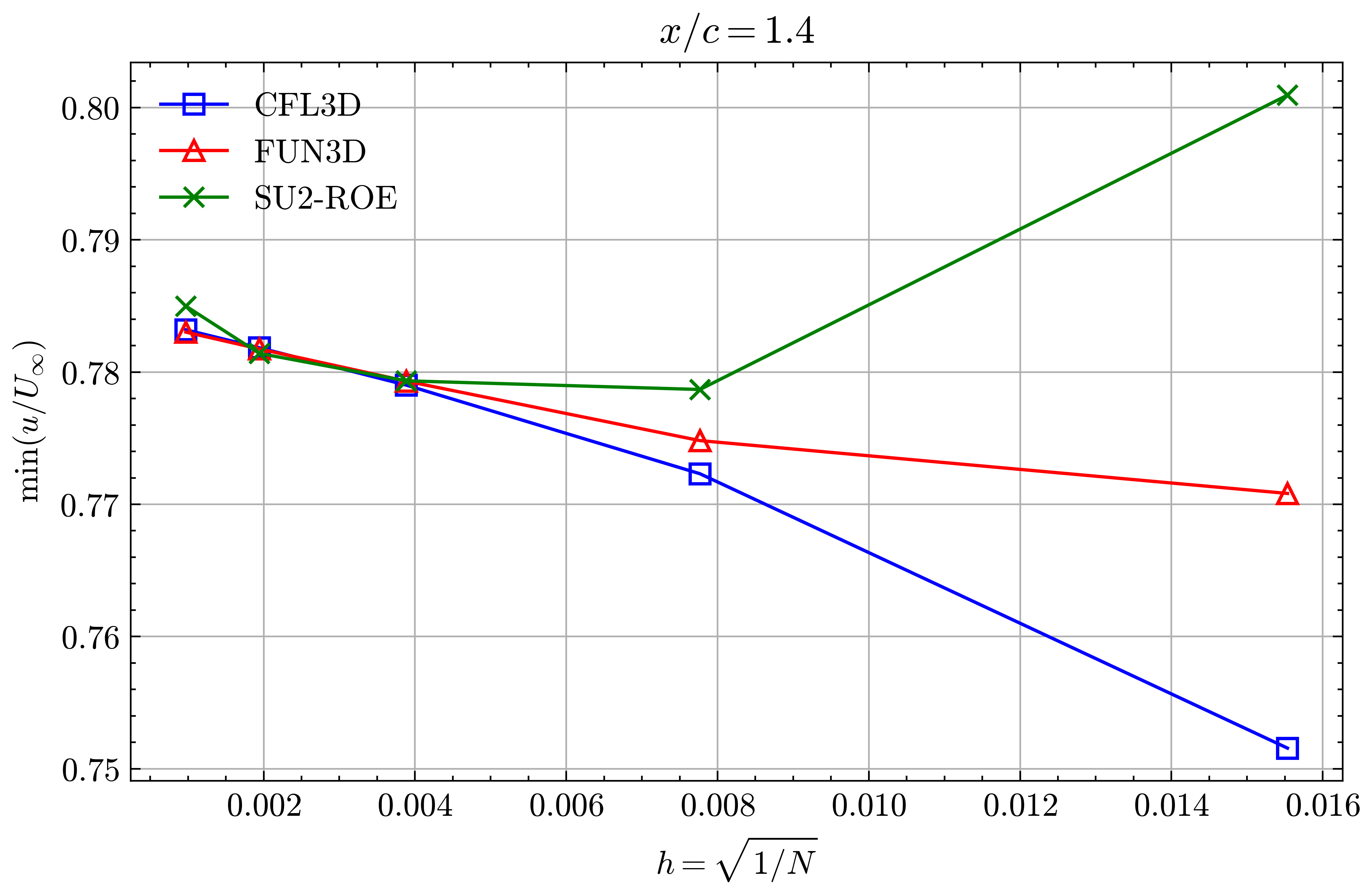
Figure (19): Min x-velocity in Wake profile grid convergence at x/c=1.40

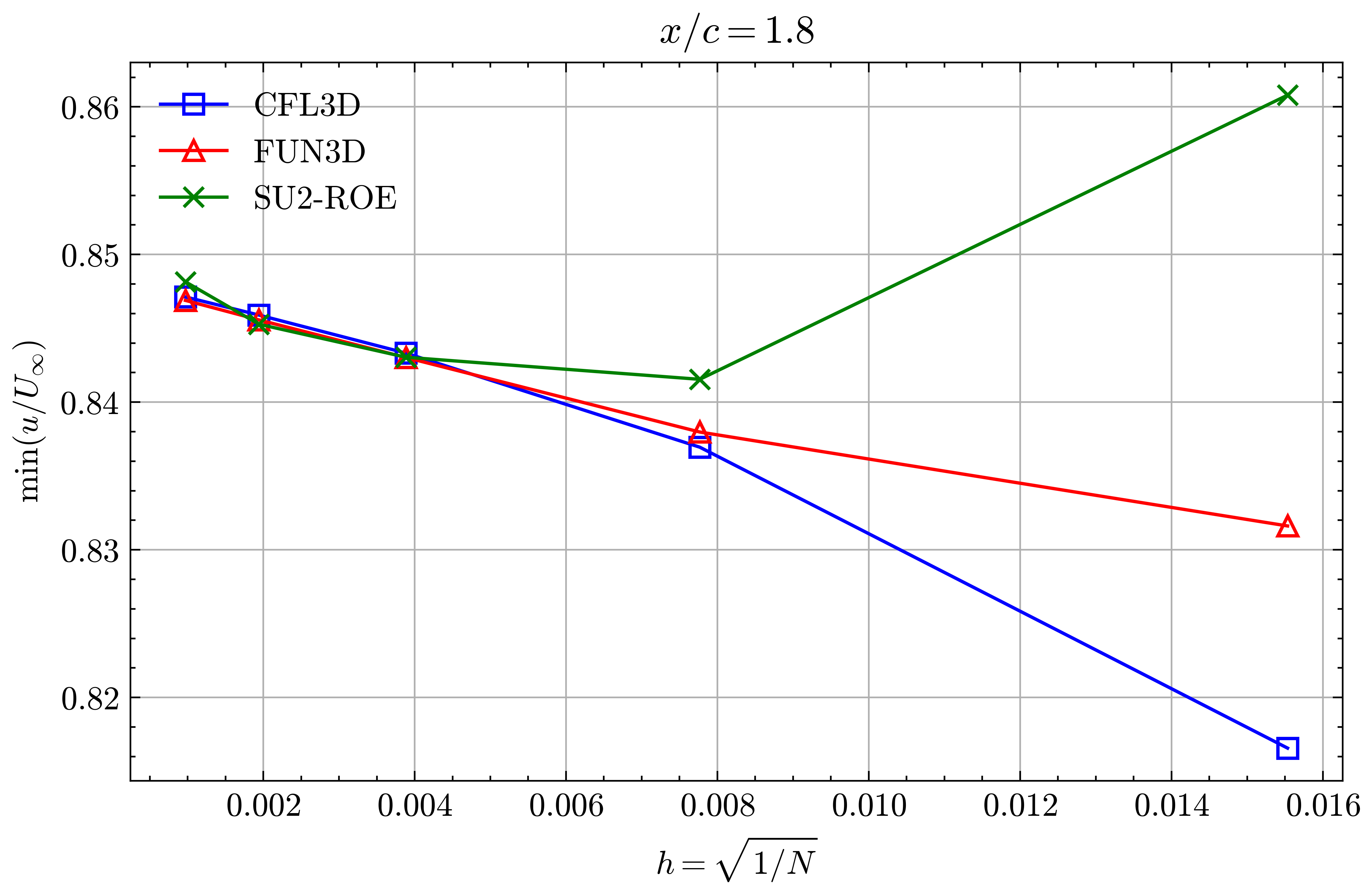
Figure (20): Min x-velocity in Wake profile grid convergence at x/c=1.80

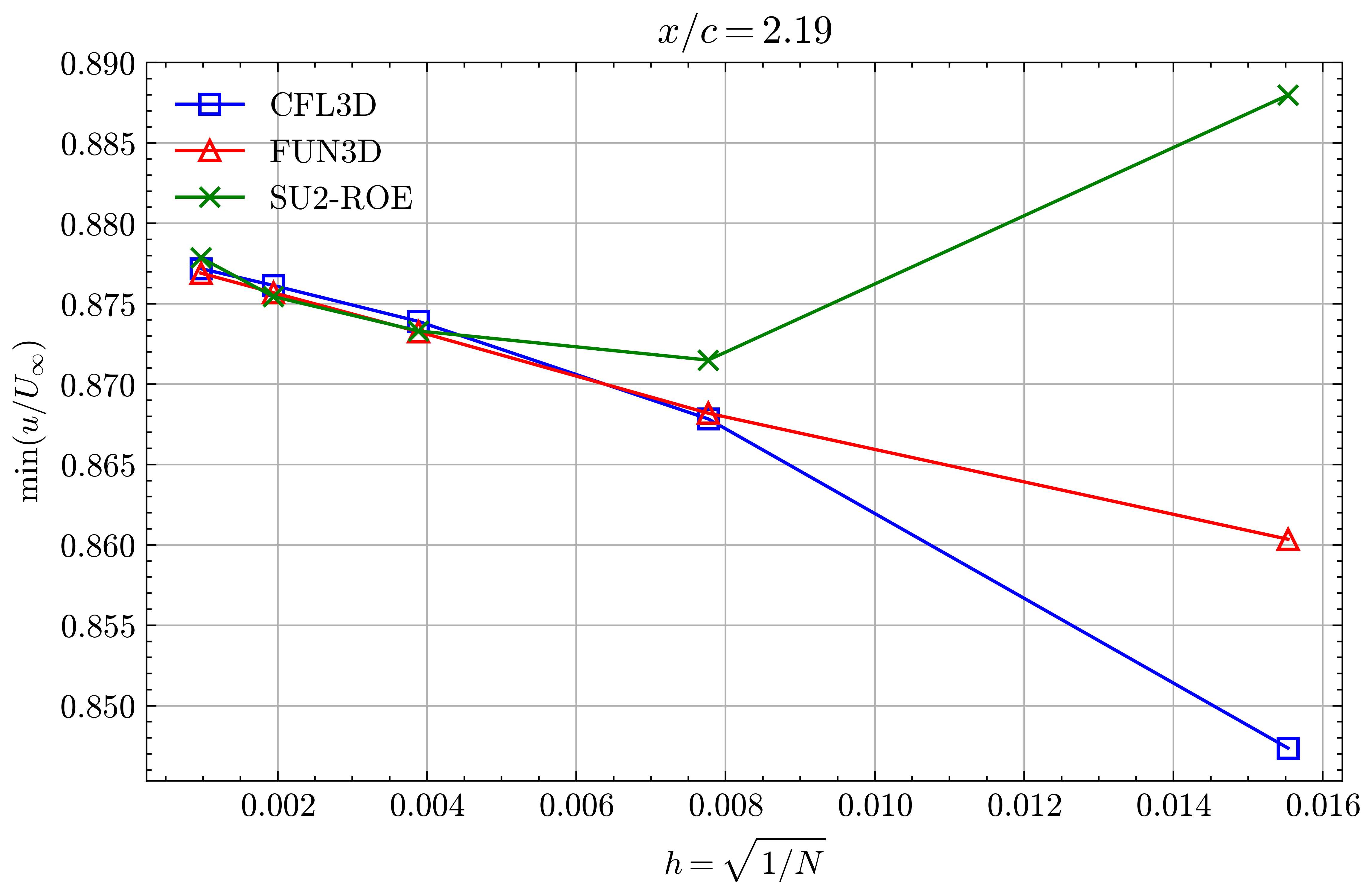
Figure (21): Min x-velocity in Wake profile grid convergence at x/c=2.19

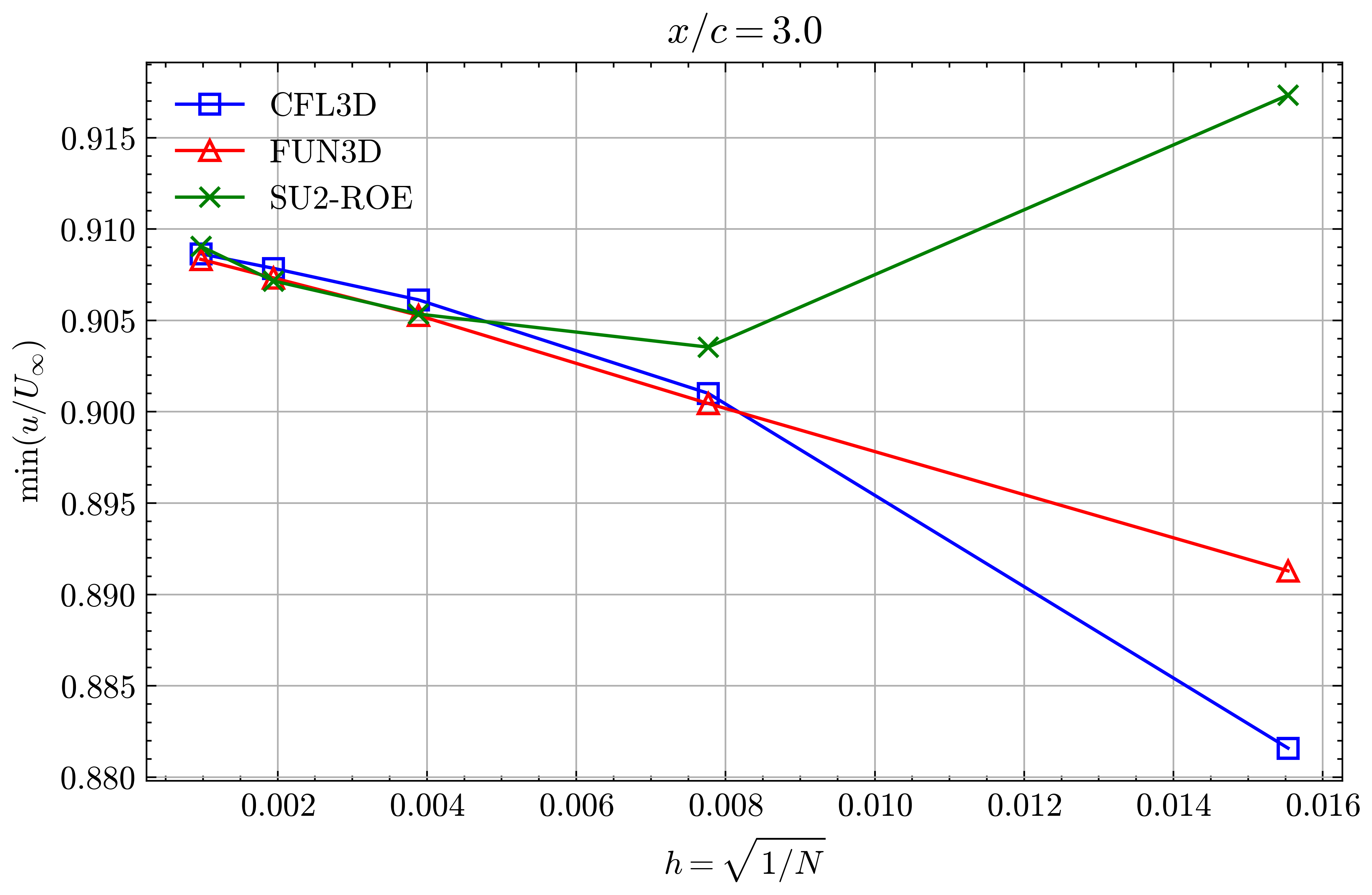
Figure (22): Min x-velocity in Wake profile grid convergence at x/c=3.00

Figure (23): Min x-velocity in Wake profile grid convergence at x/c=3.00

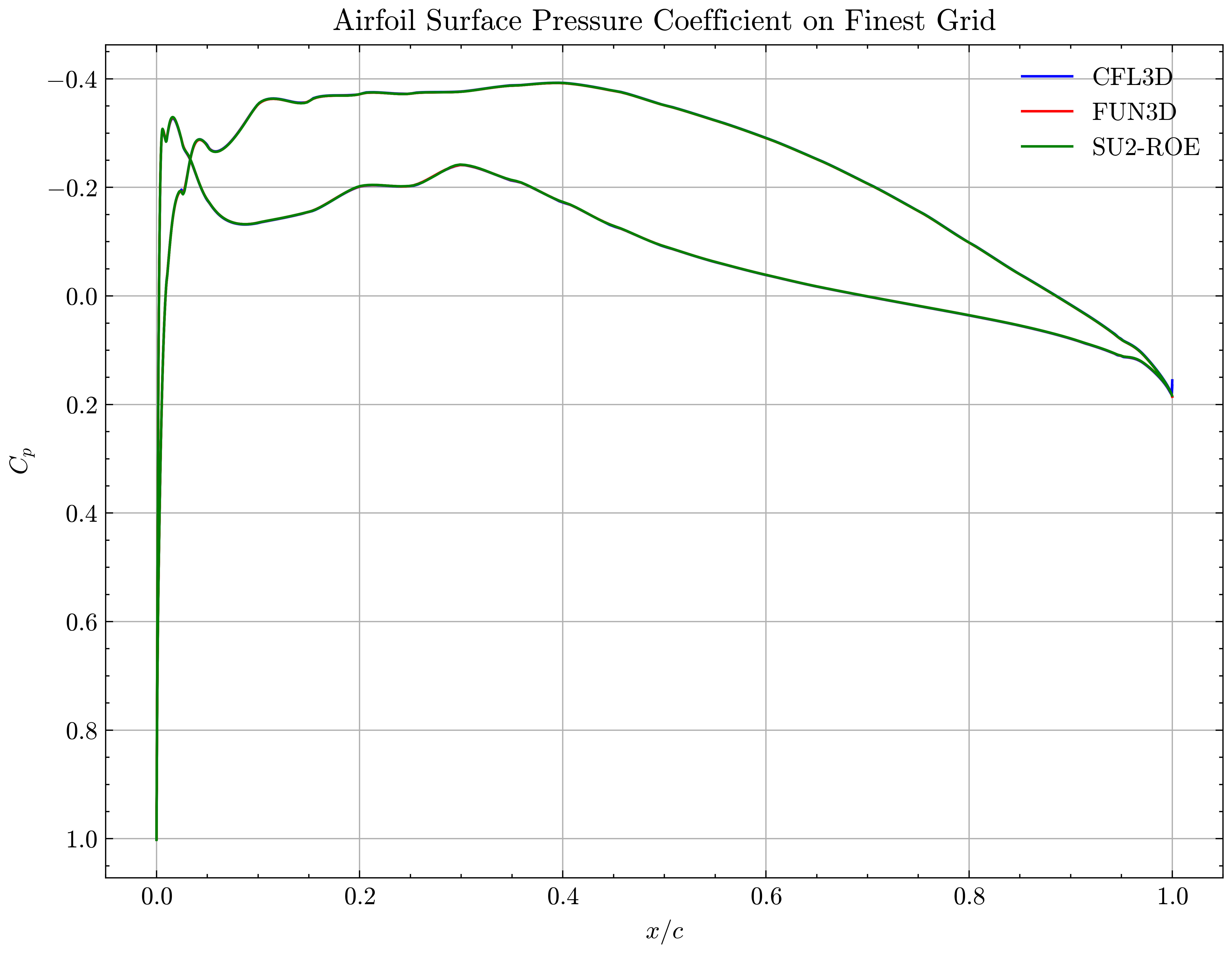
Figure (24): Airfoil Surface Pressure Coefficient on Finest Grid

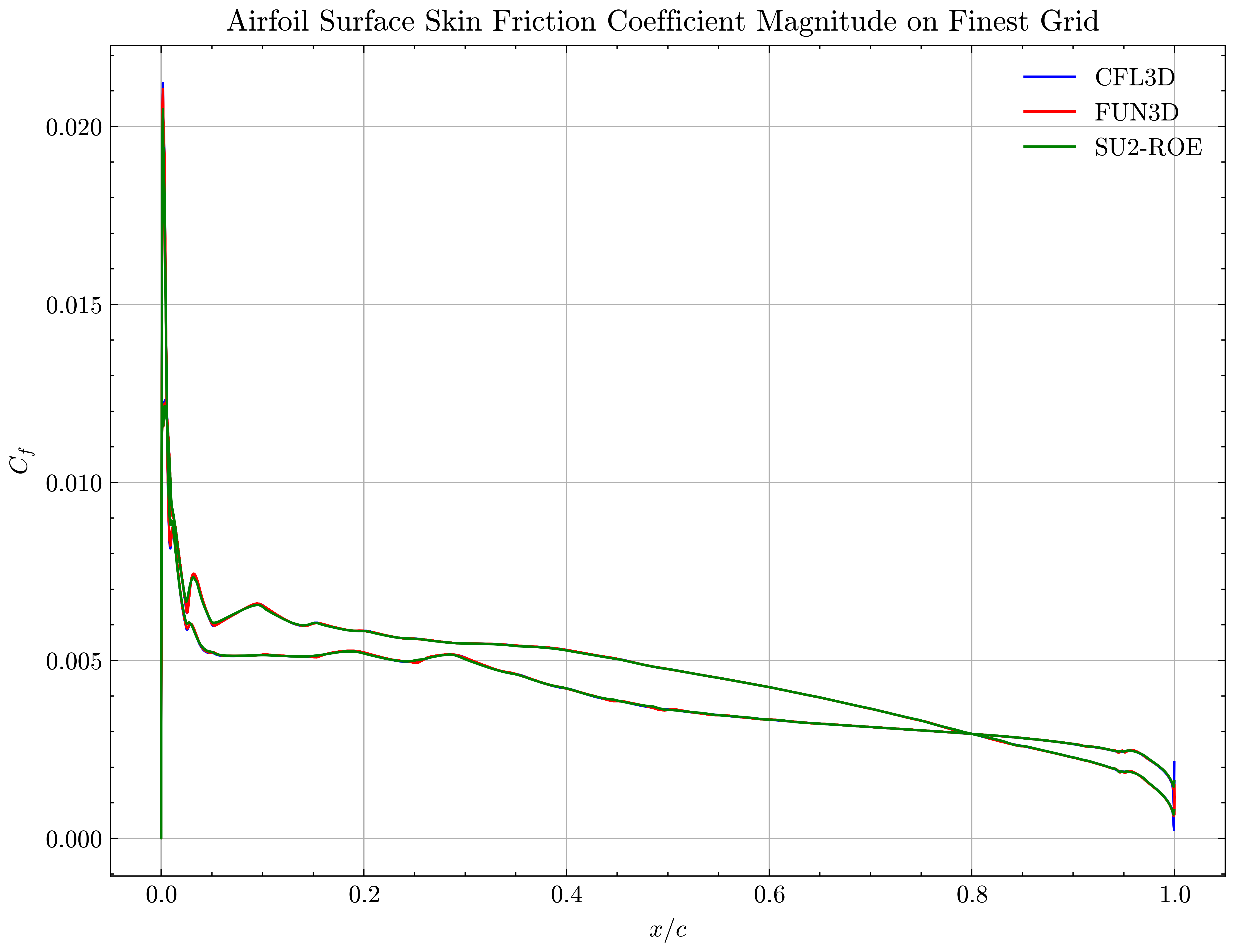
Figure (25): Airfoil Surface Skin Friction Coefficient on Finest Grid

SST Model

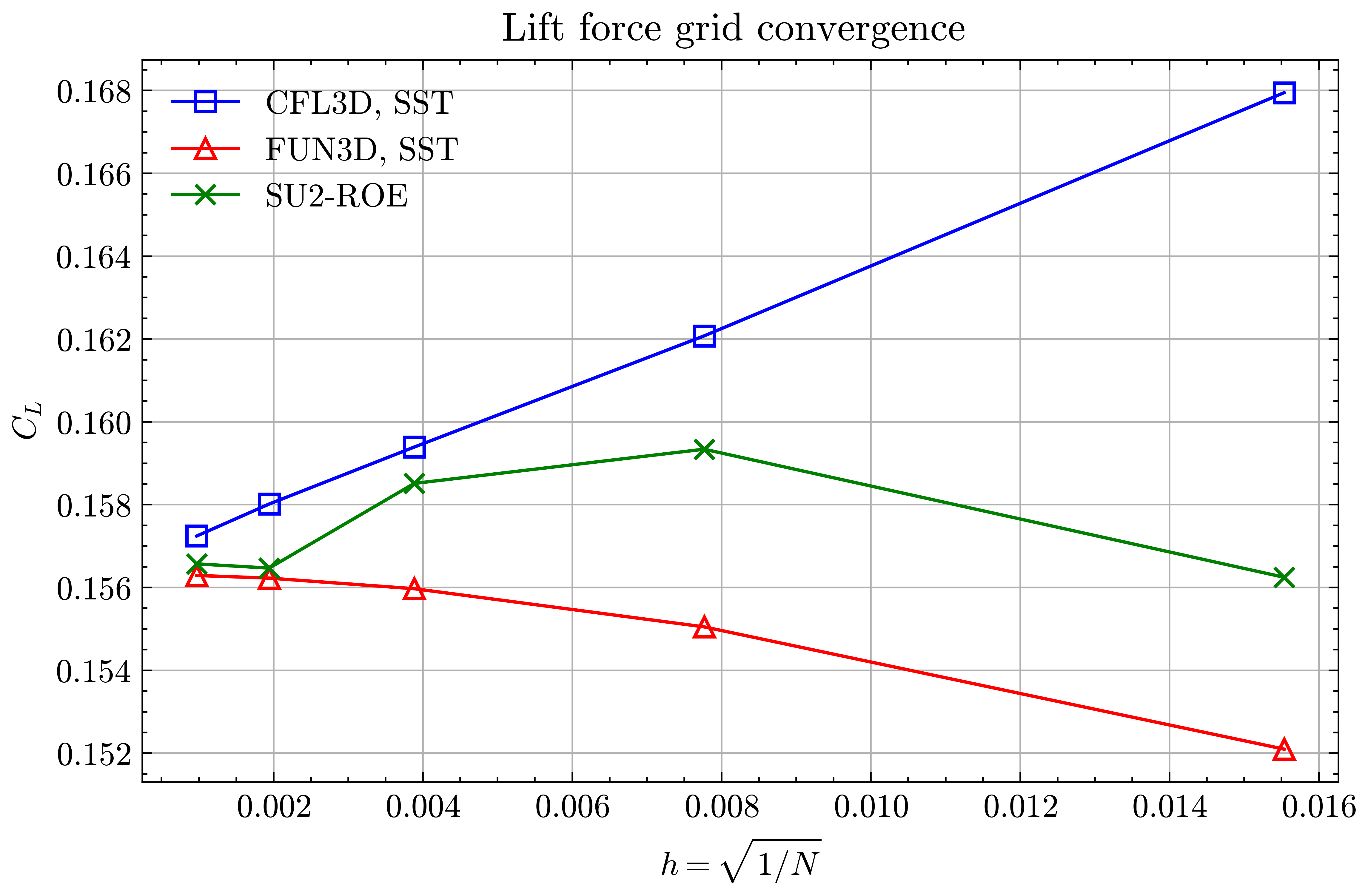
Figure (26): Lift force grid convergence

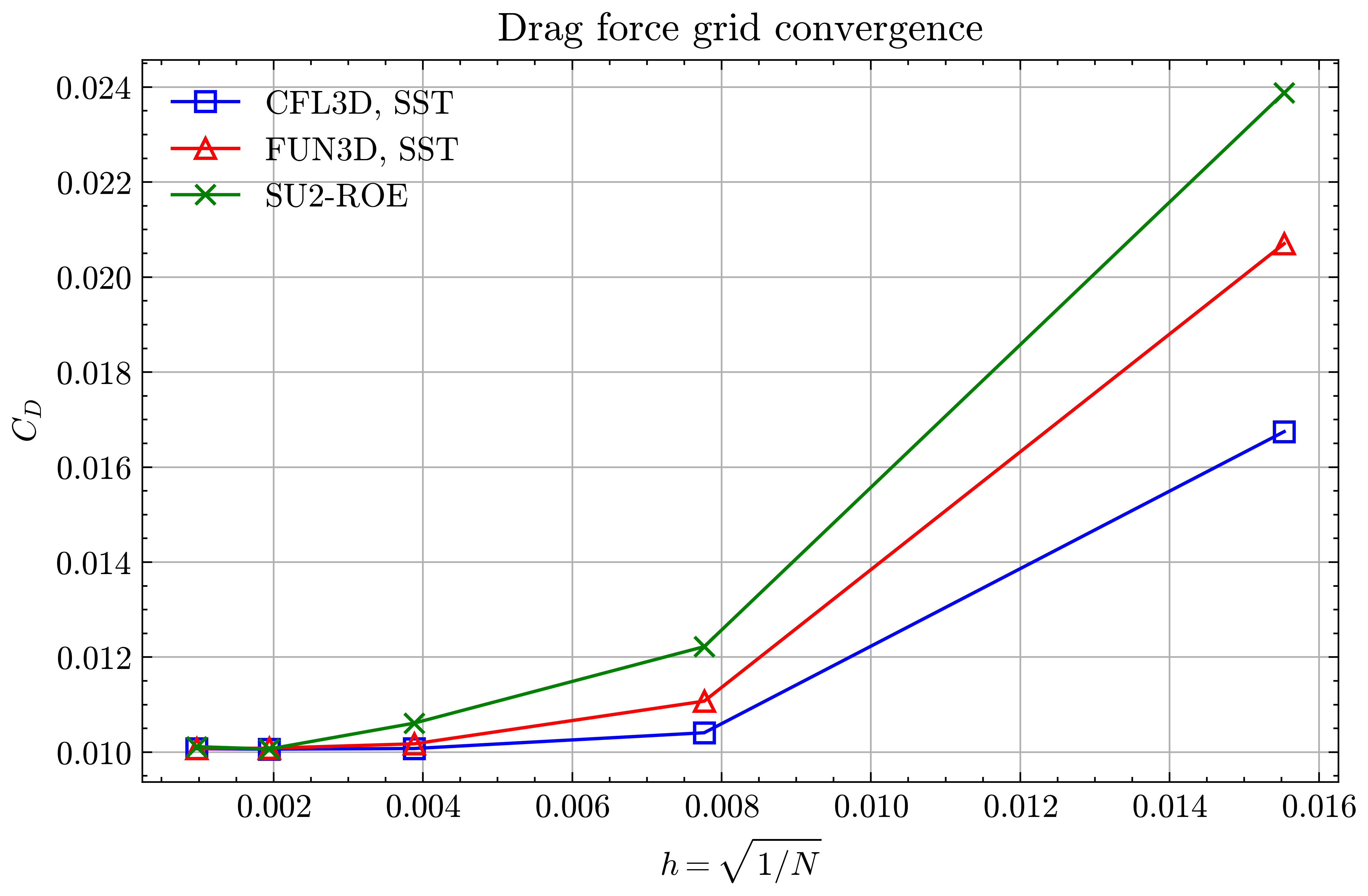
Figure (27): Drag force grid convergence

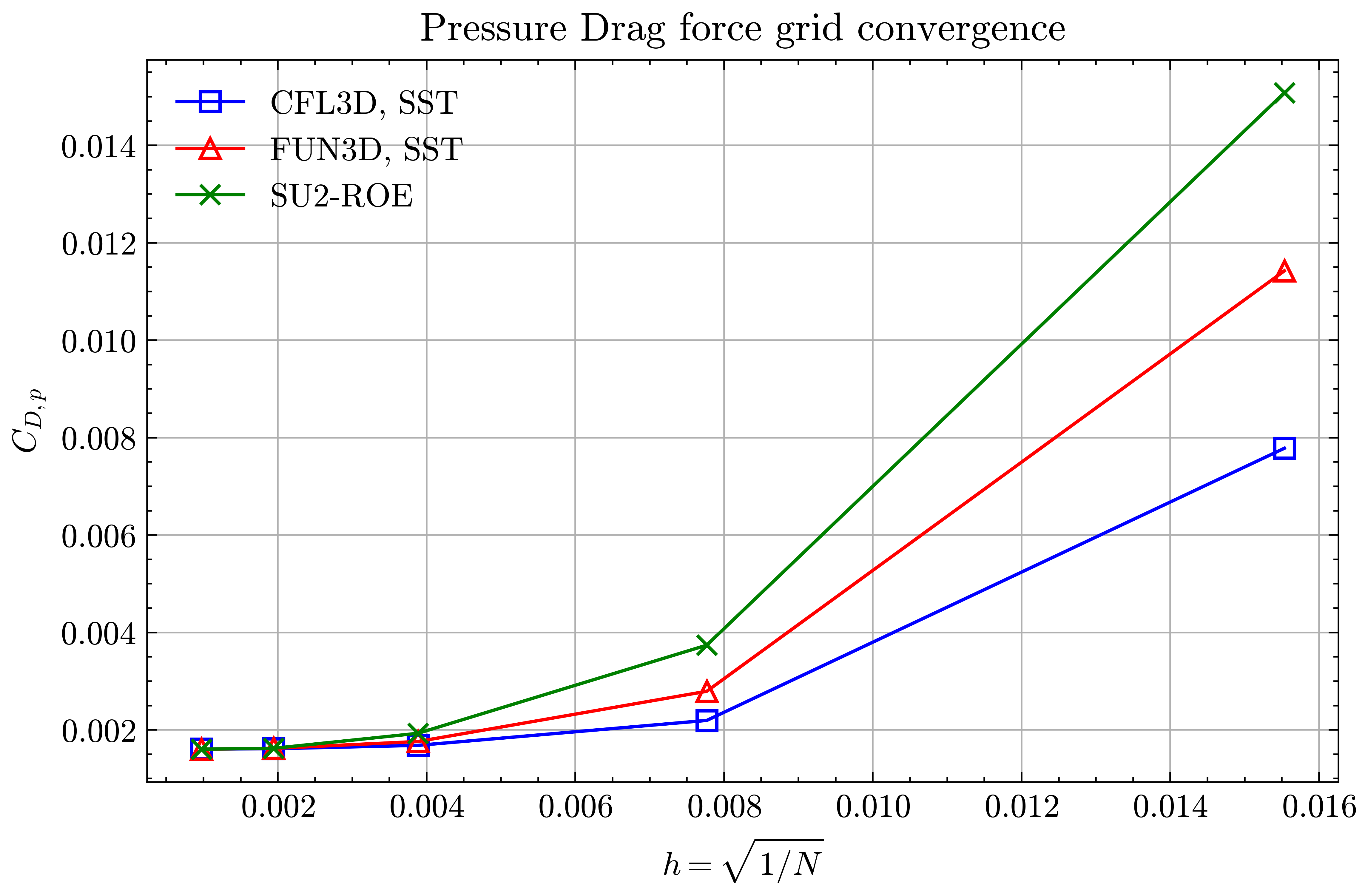
Figure (28): Pressure Drag force grid convergence

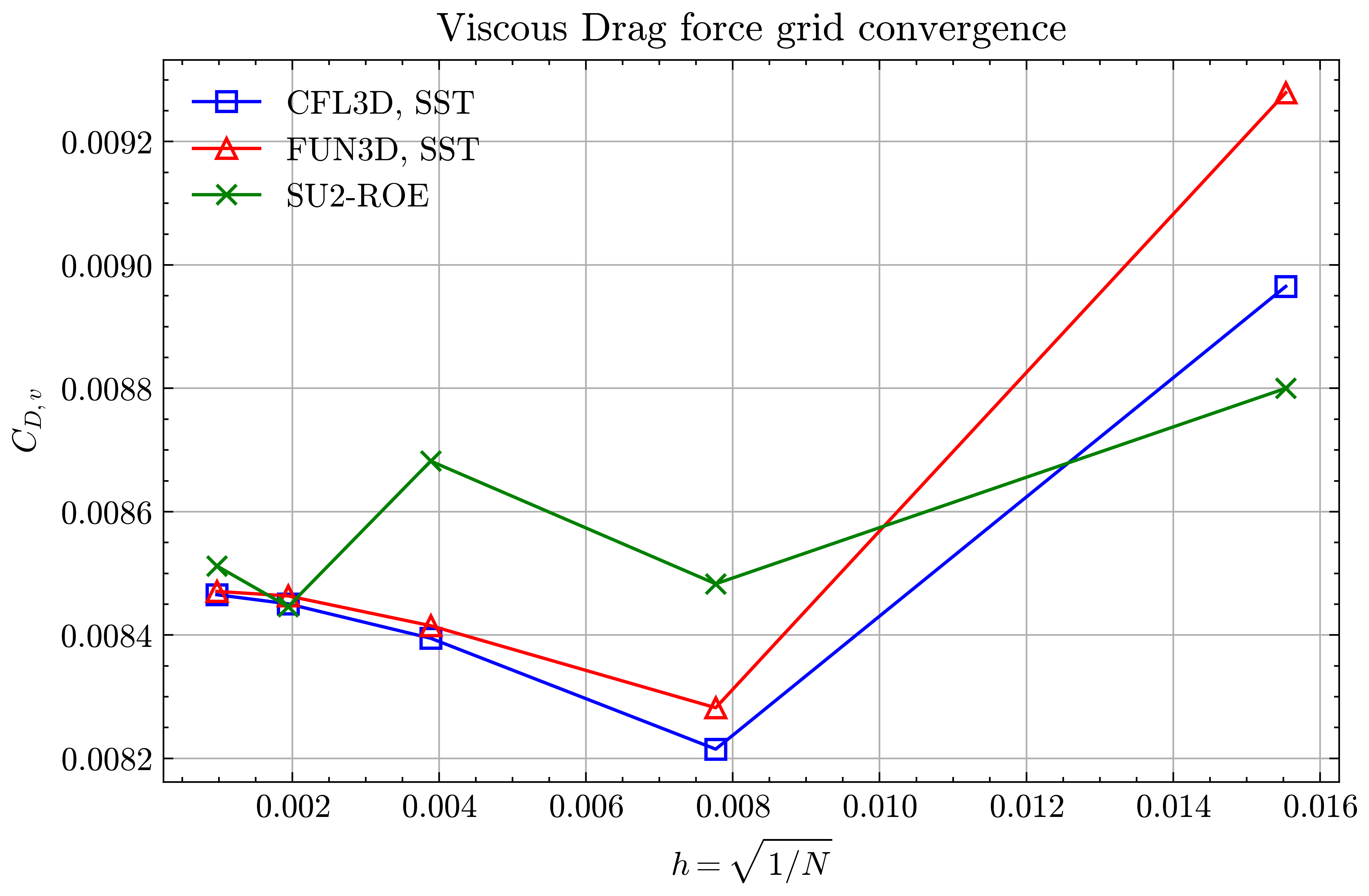
Figure (29): Viscous Drag force grid convergence

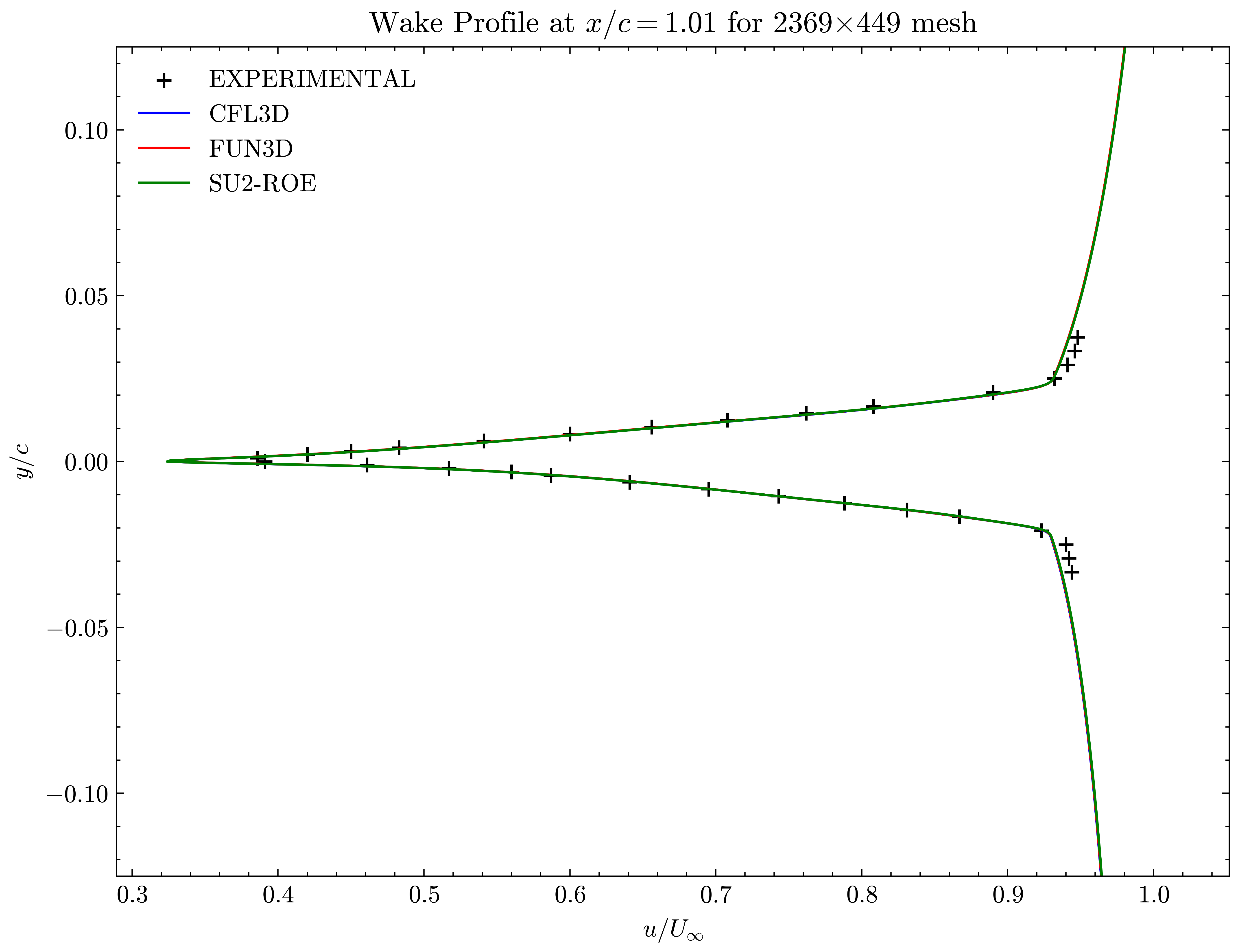
Figure (30): Wake profile at x/c=1.01

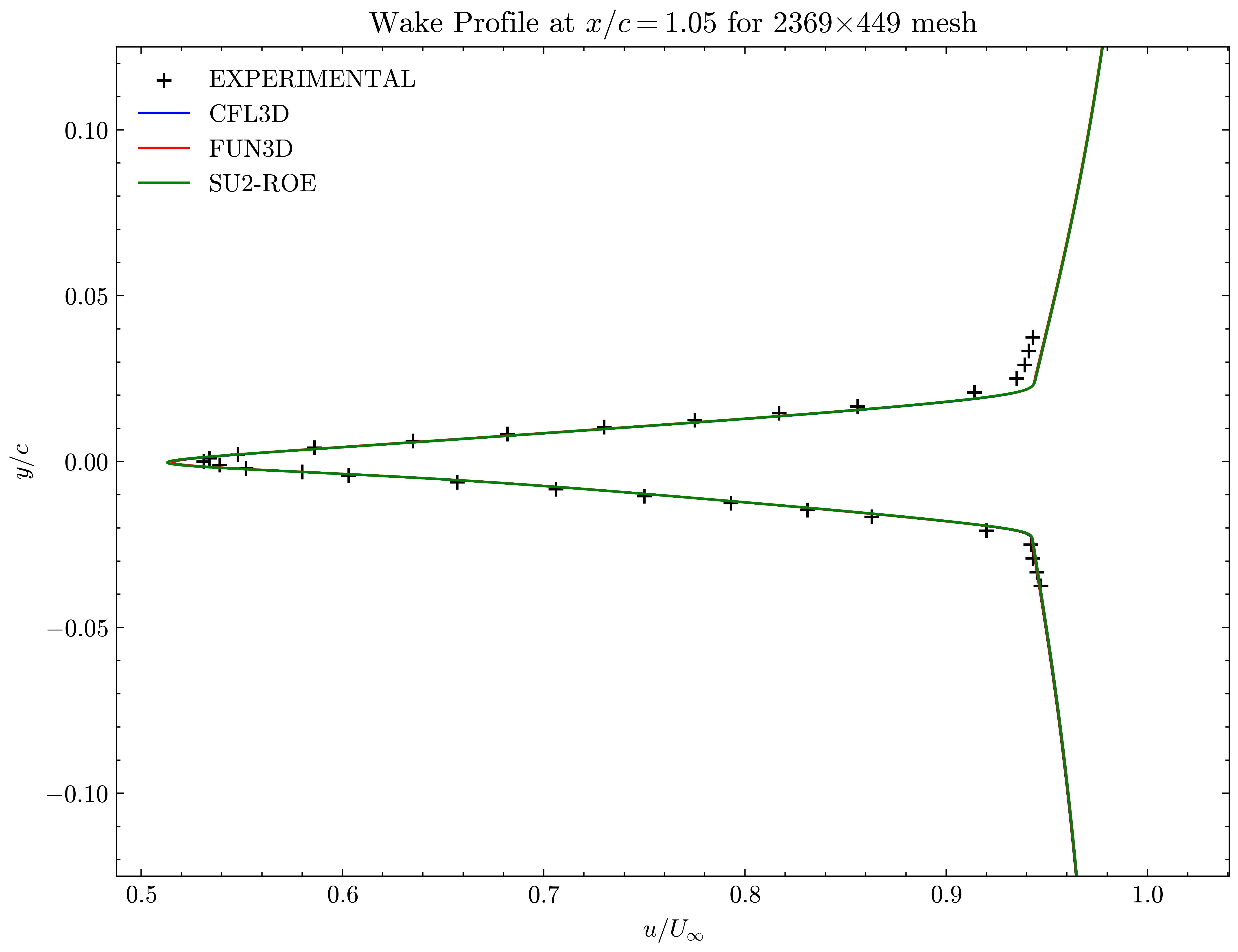
Figure (31): Wake profile at x/c=1.05

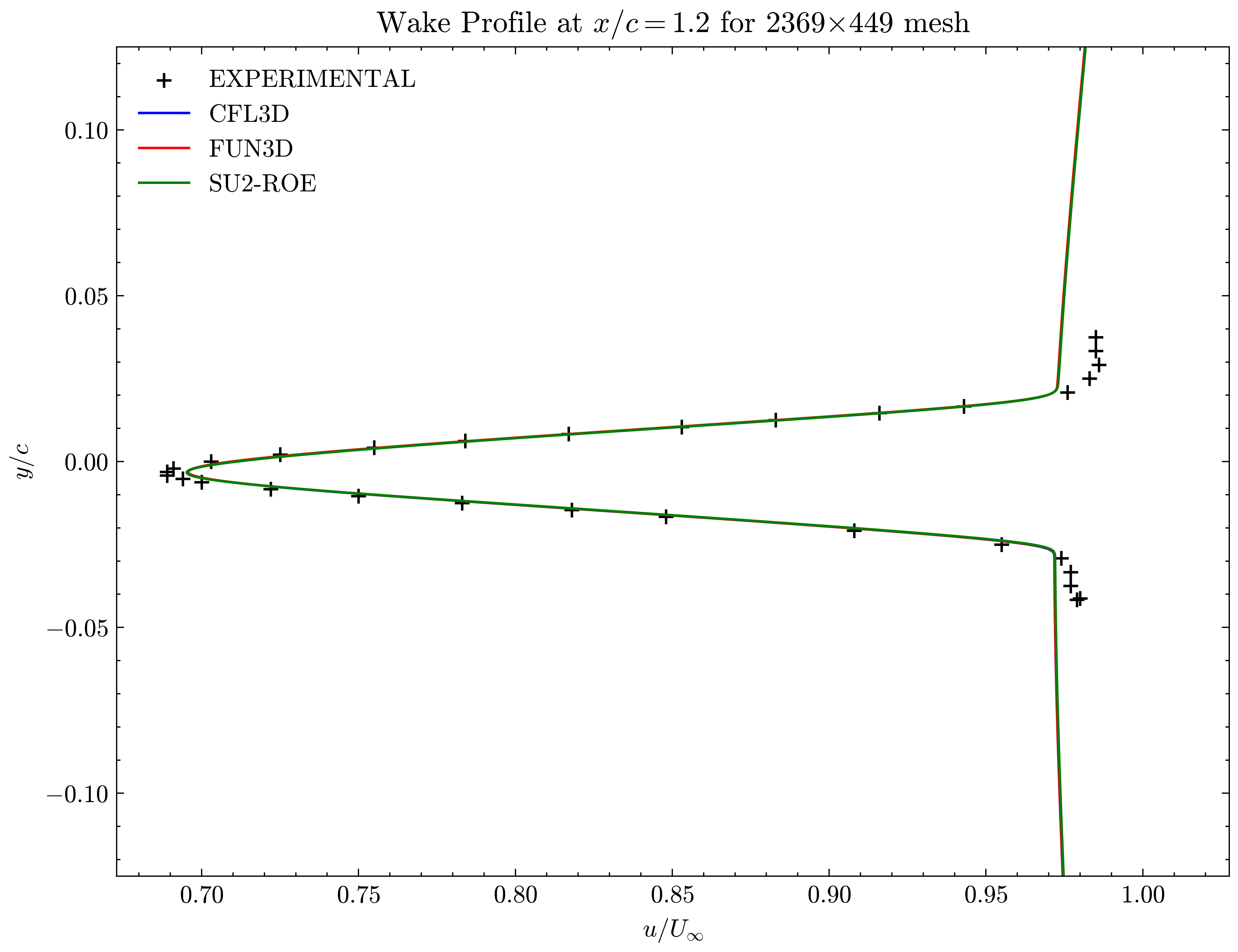
Figure (32): Wake profile at x/c=1.20

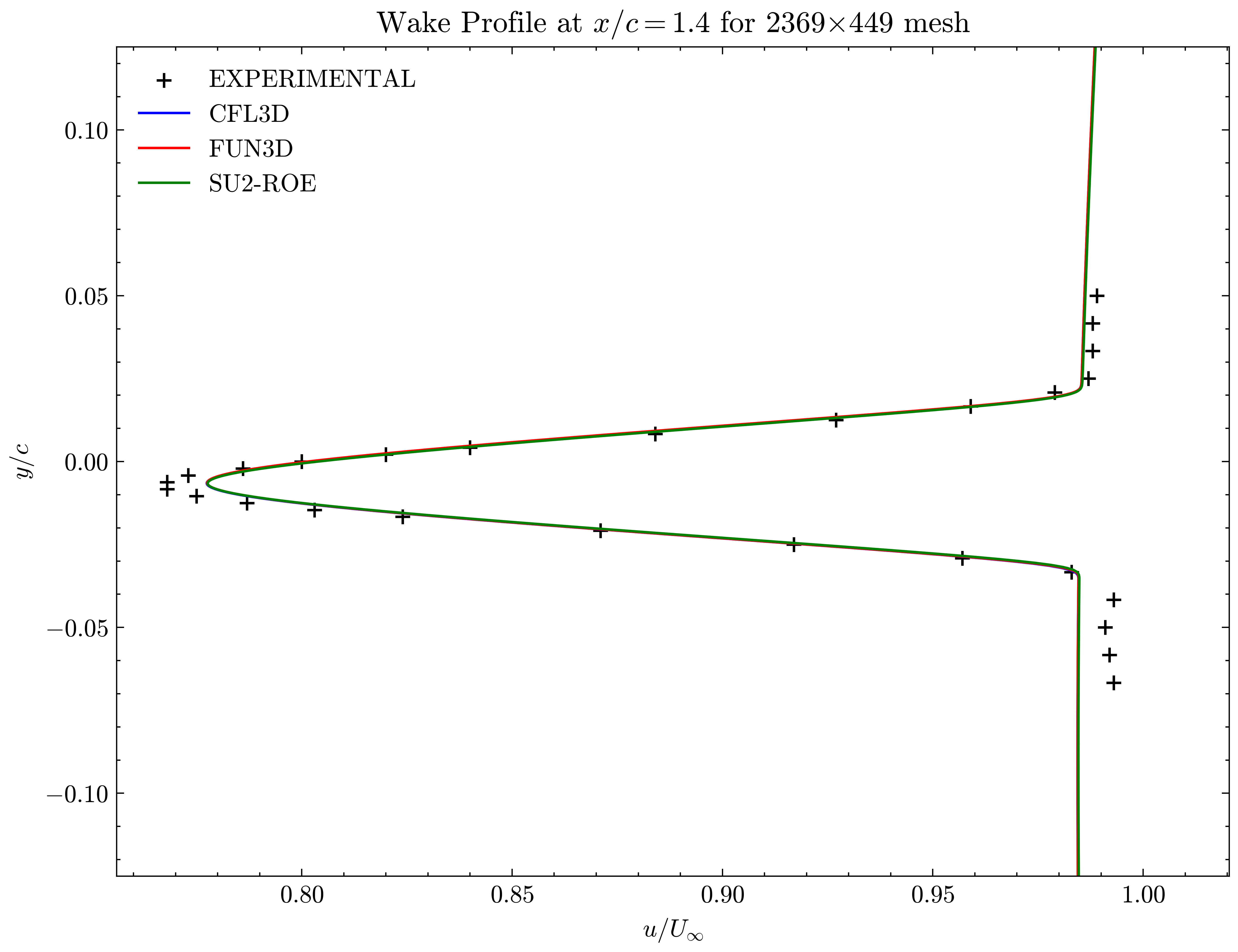
Figure (33): Wake profile at x/c=1.40

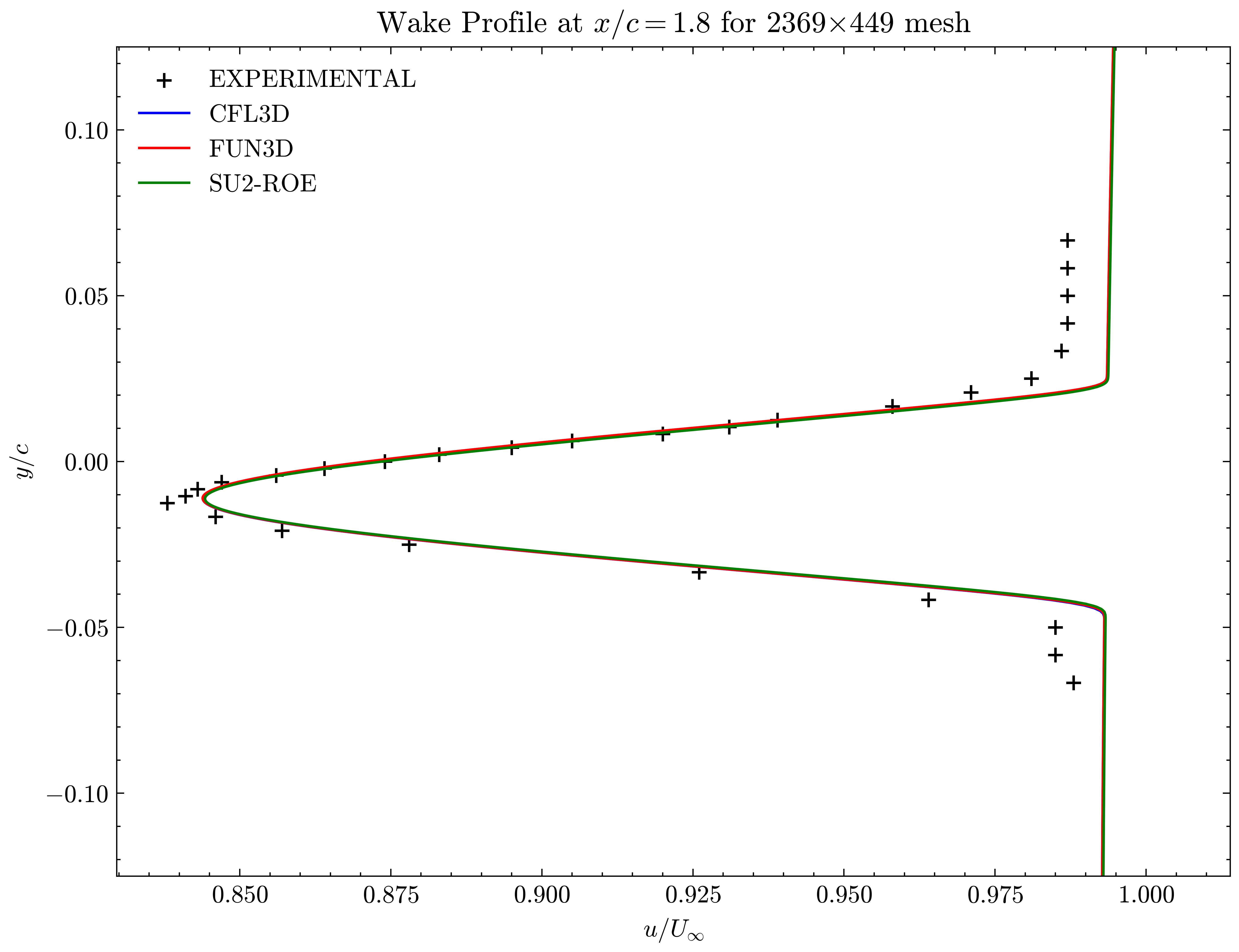
Figure (34): Wake profile at x/c=1.80

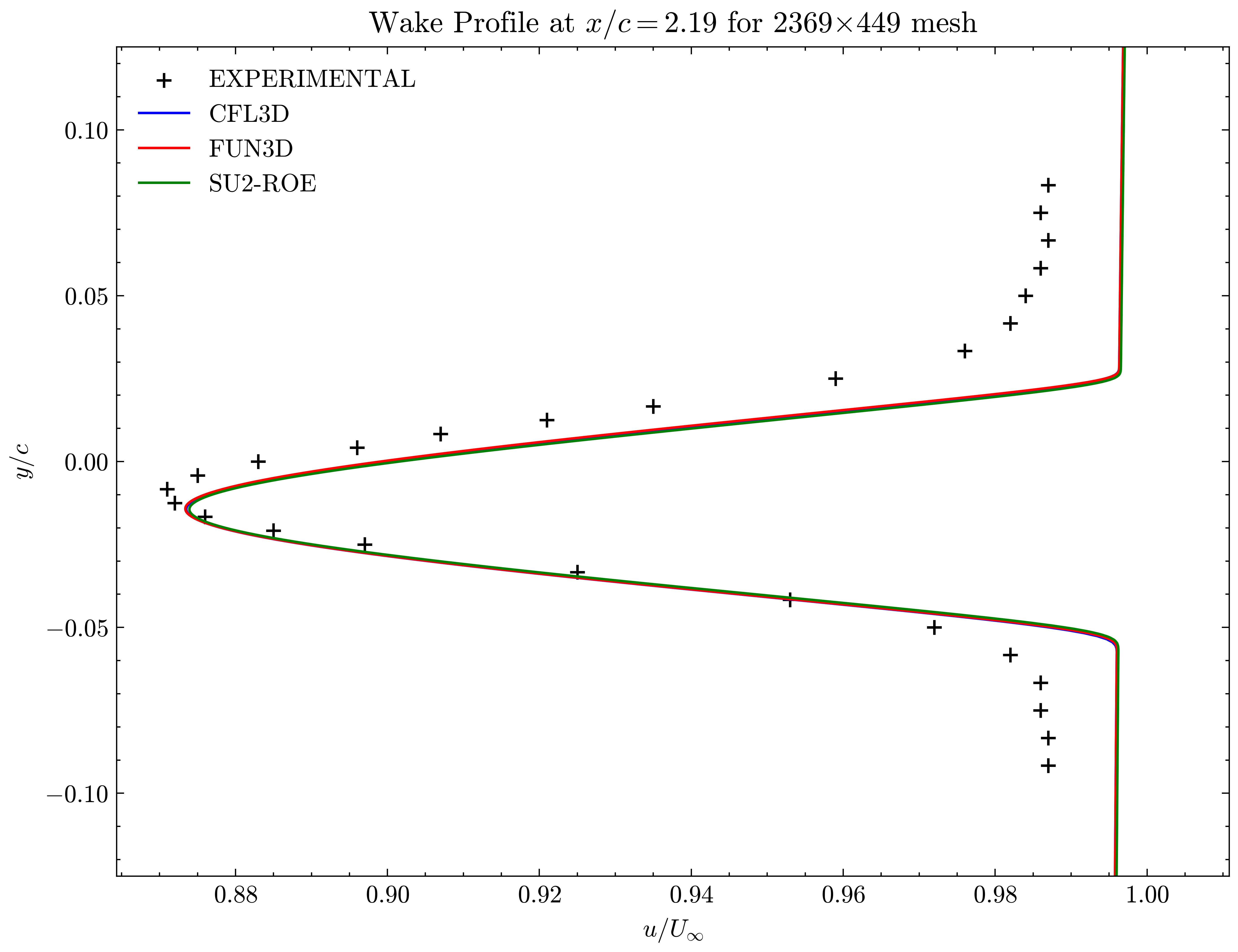
Figure (35): Wake profile at x/c=2.19

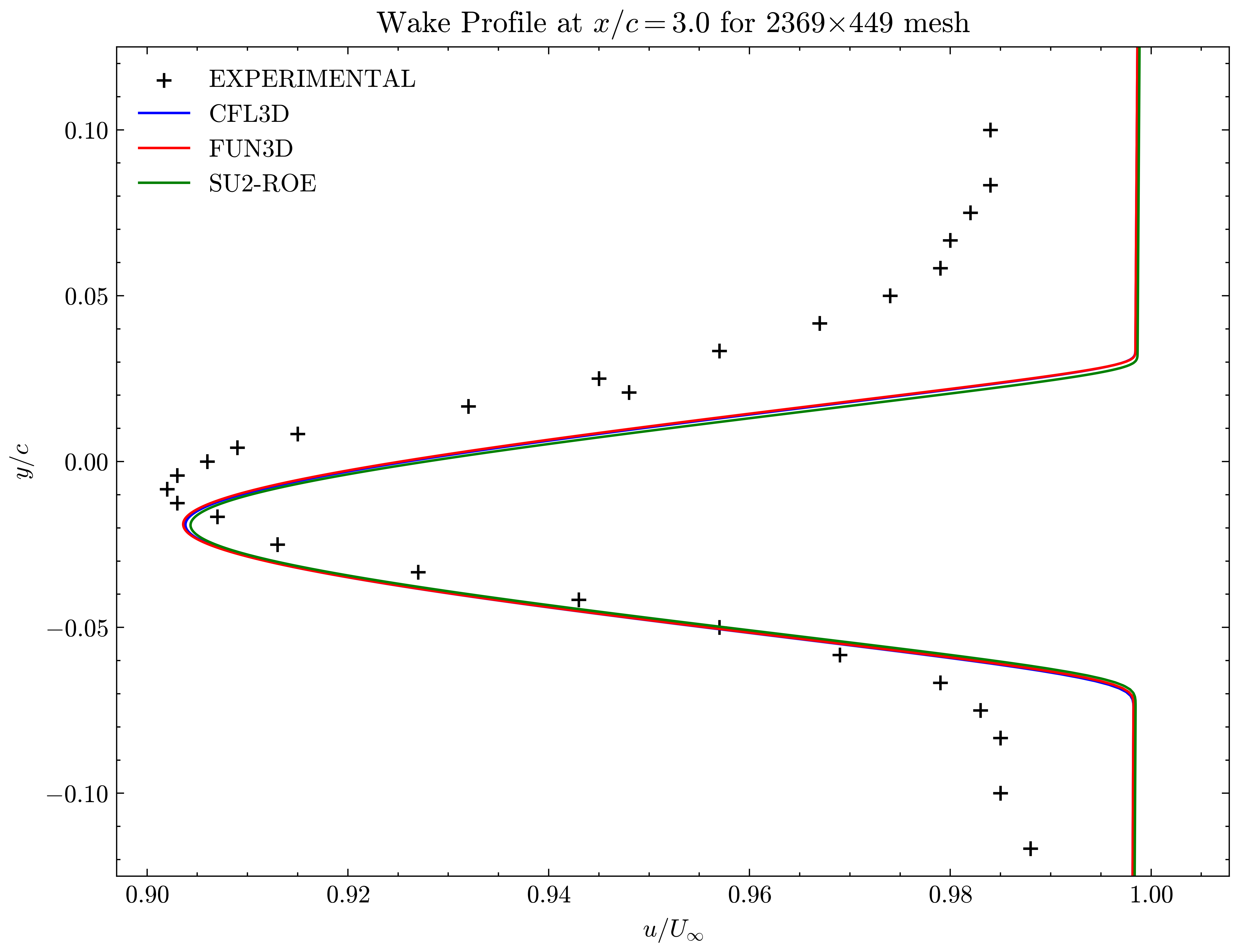
Figure (36): Wake profile at x/c=3.00

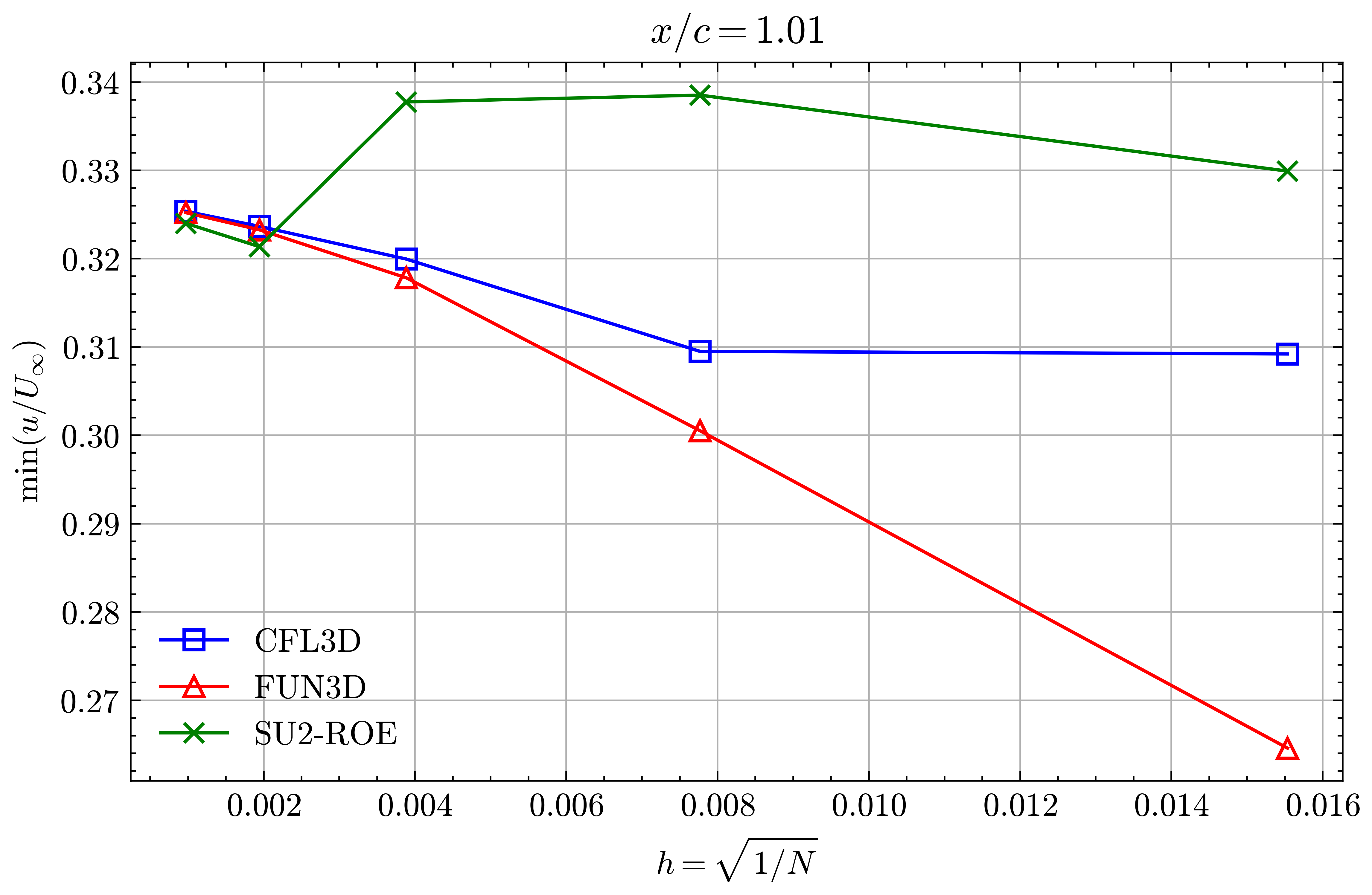
Figure (37): Min x-velocity in Wake profile grid convergence at x/c=1.01

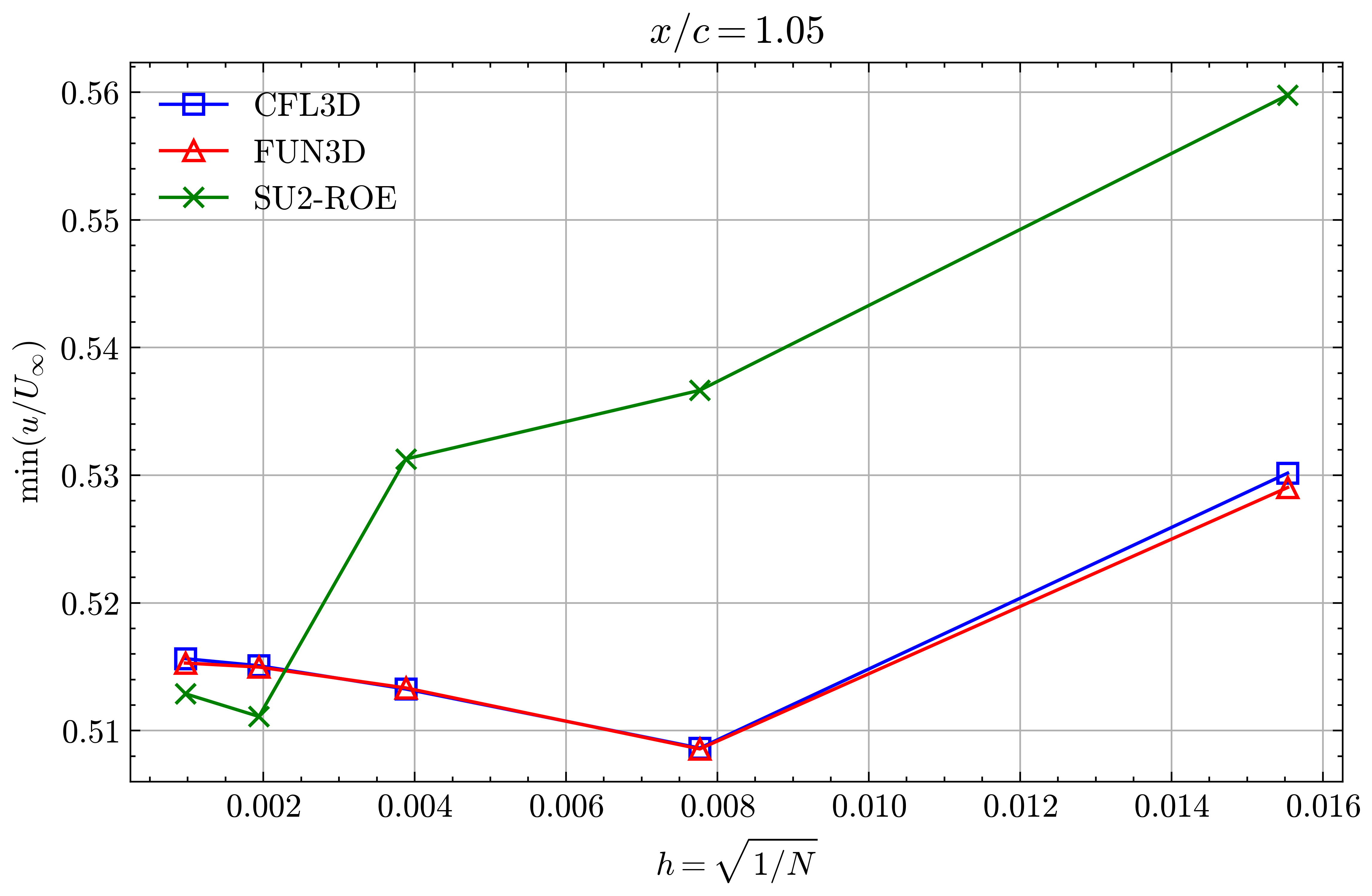
Figure (38): Min x-velocity in Wake profile grid convergence at x/c=1.05

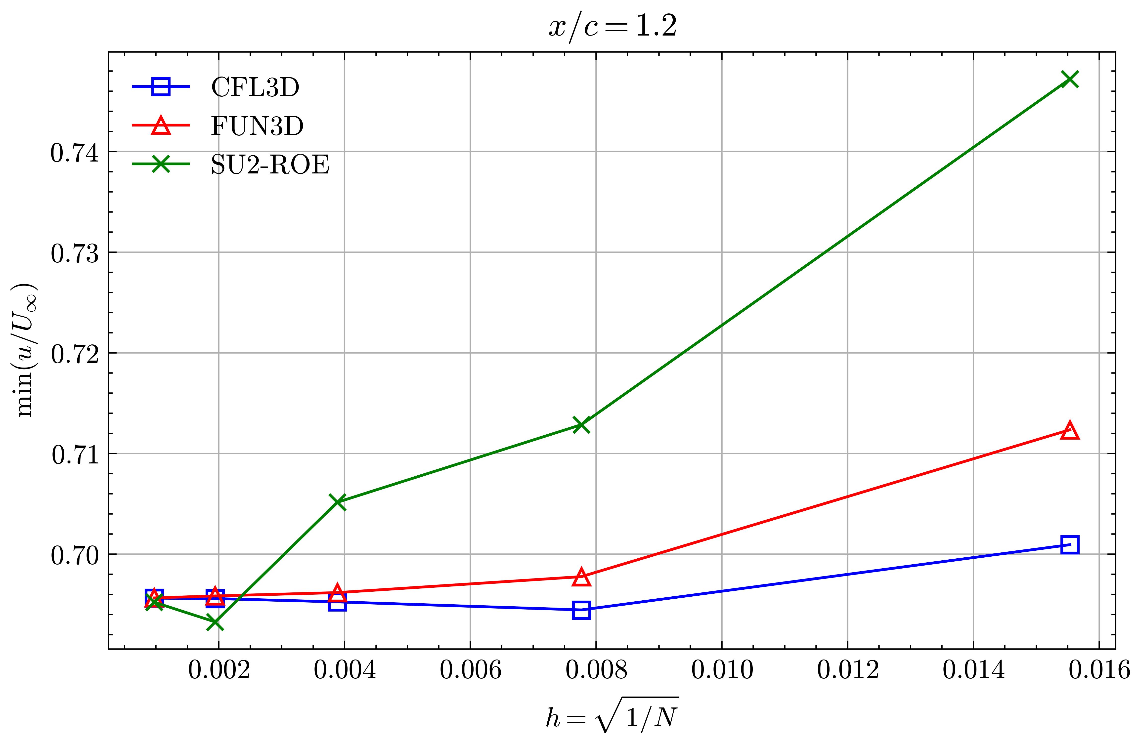
Figure (39): Min x-velocity in Wake profile grid convergence at x/c=1.20

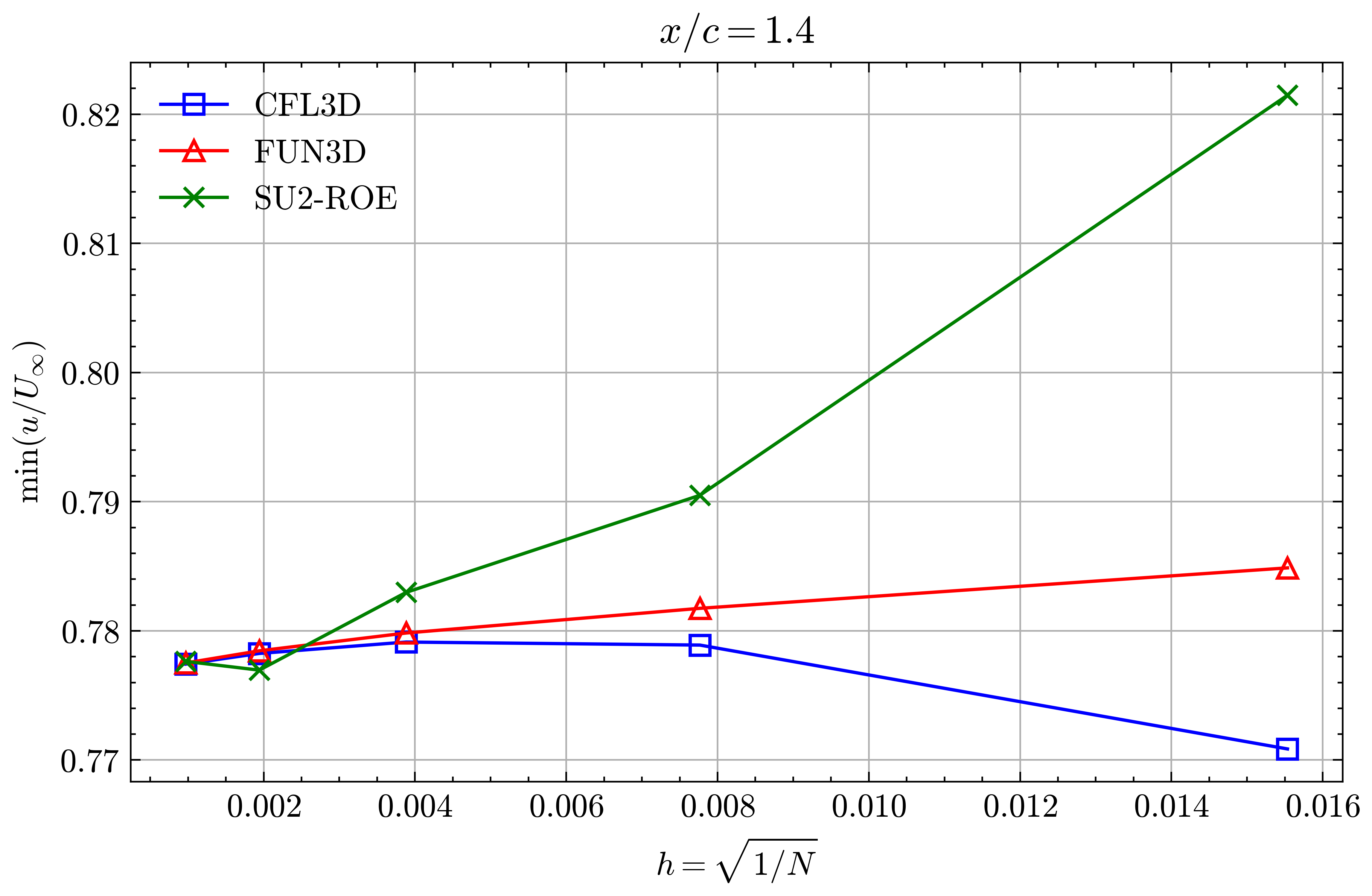
Figure (40): Min x-velocity in Wake profile grid convergence at x/c=1.40

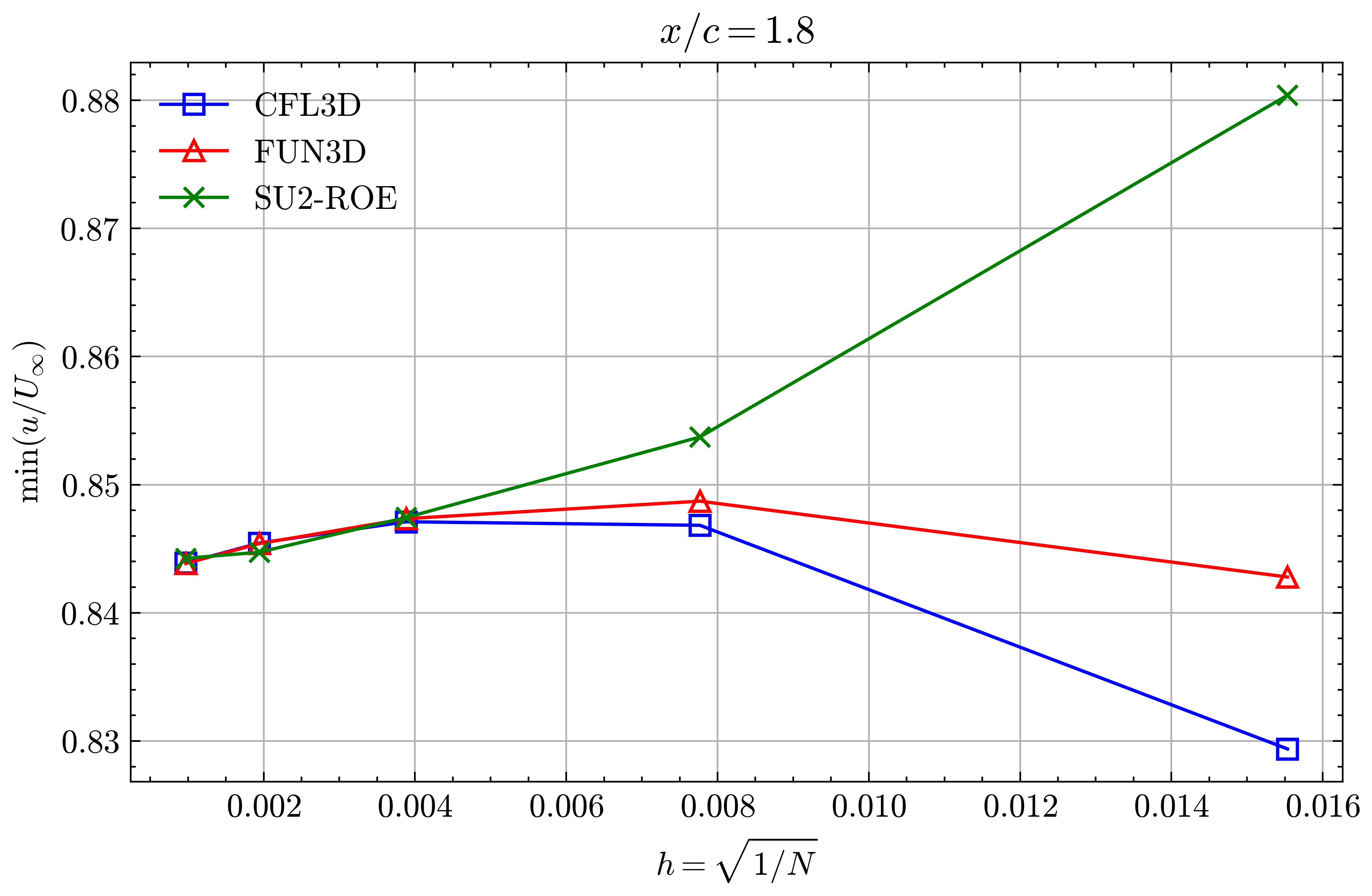
Figure (41): Min x-velocity in Wake profile grid convergence at x/c=1.80

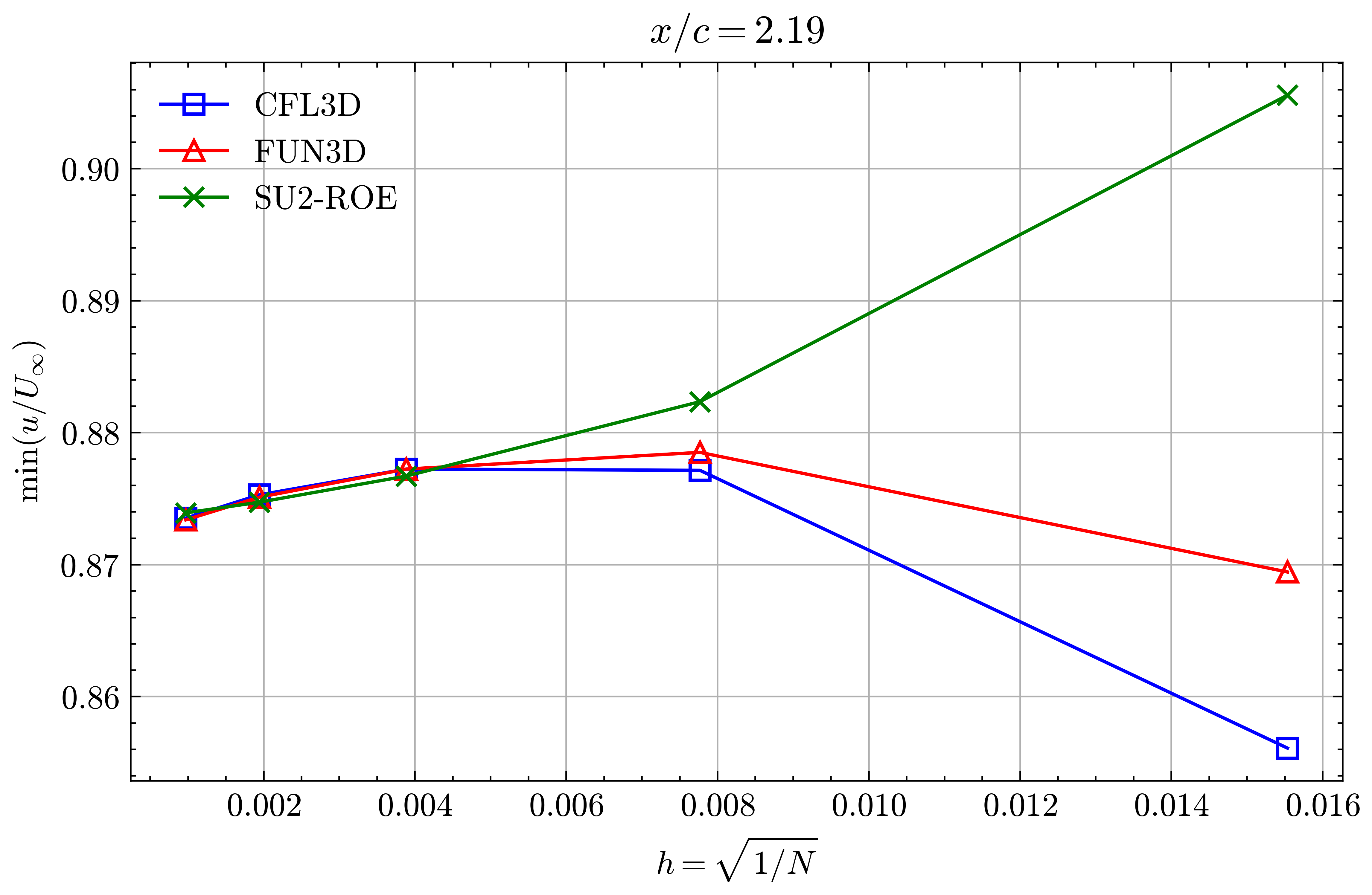
Figure (42): Min x-velocity in Wake profile grid convergence at x/c=2.19

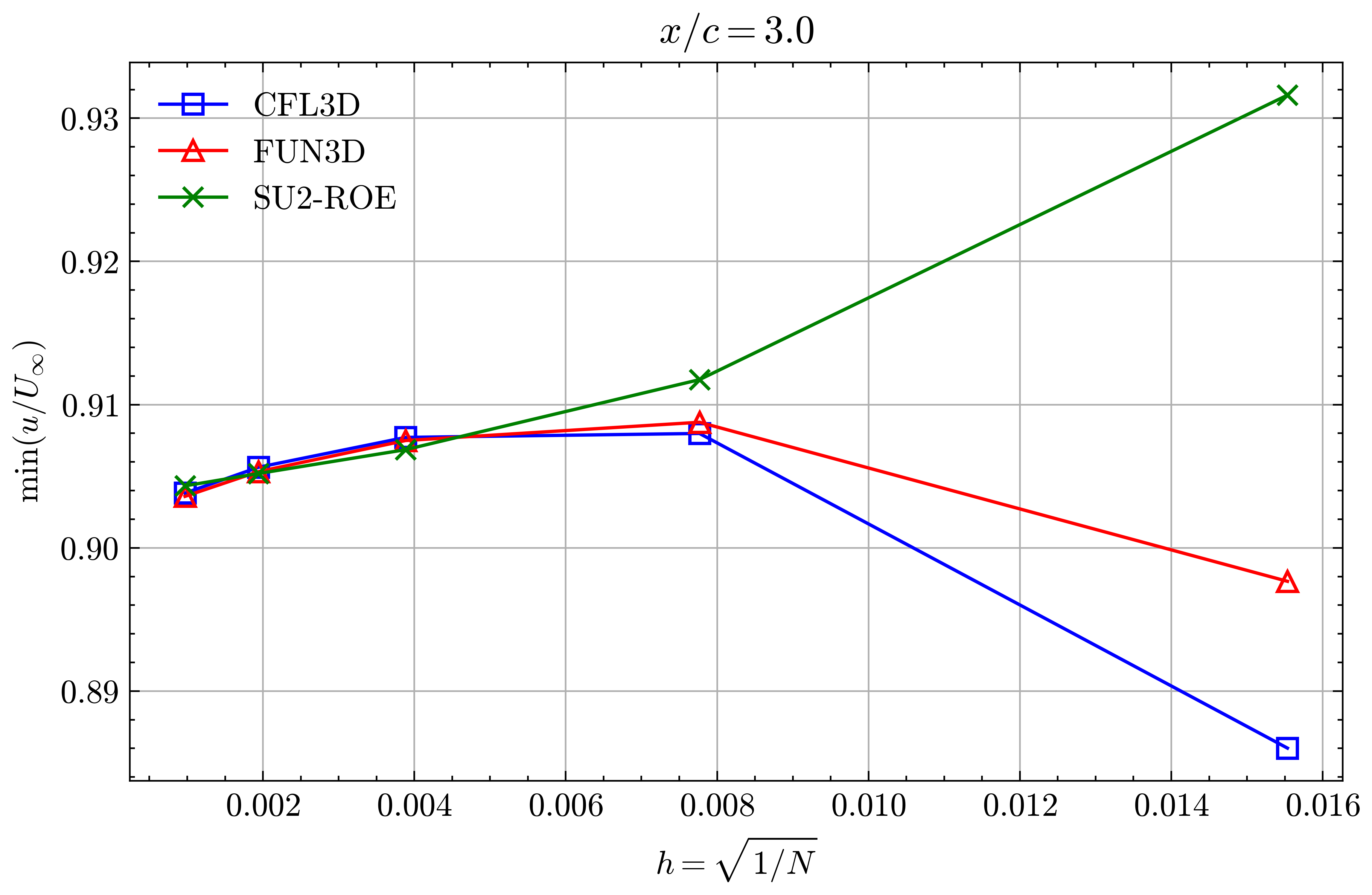
Figure (43): Min x-velocity in Wake profile grid convergence at x/c=3.00

Figure (44): Min x-velocity in Wake profile grid convergence at x/c=3.00

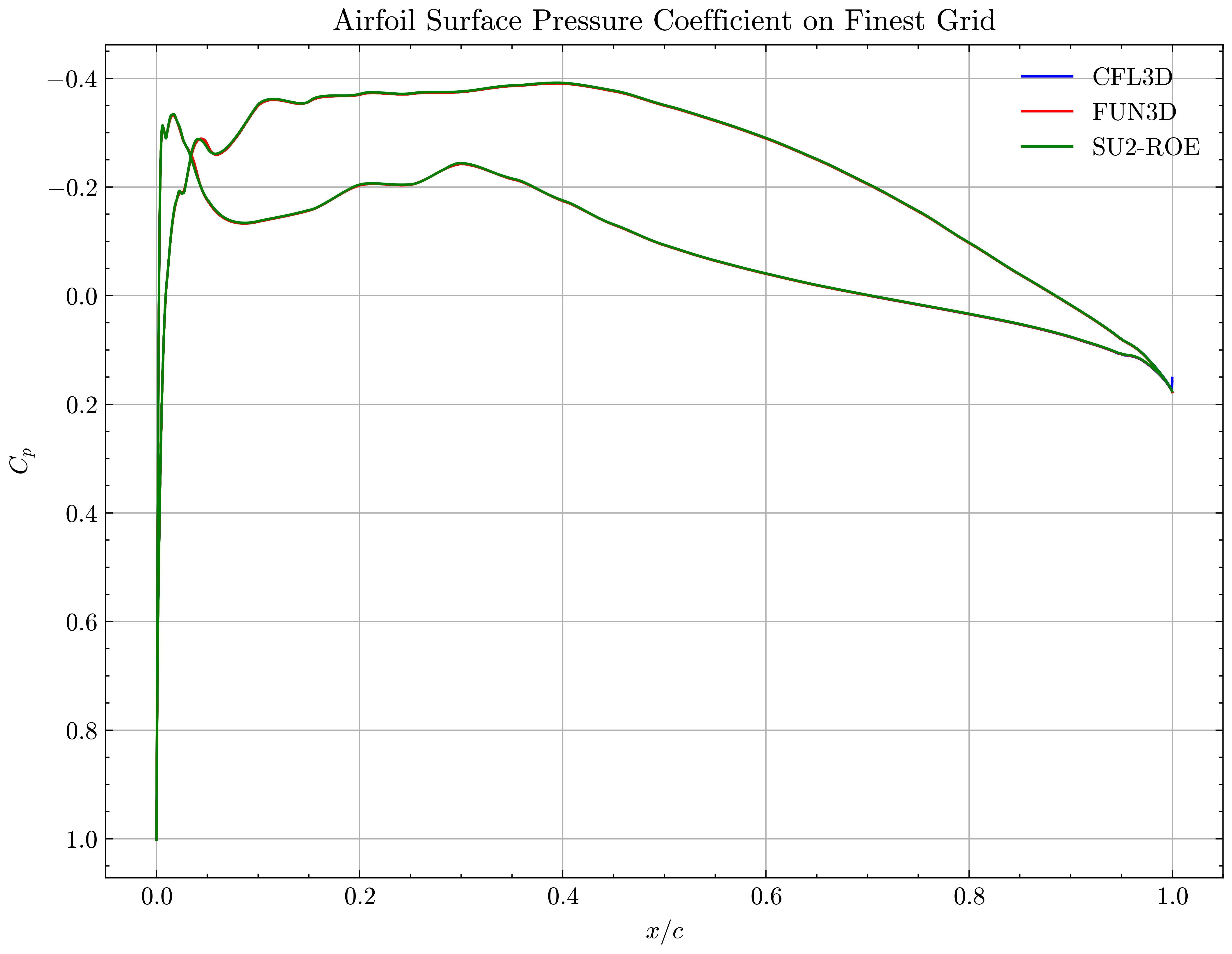
Figure (45): Airfoil Surface Pressure Coefficient on Finest Grid

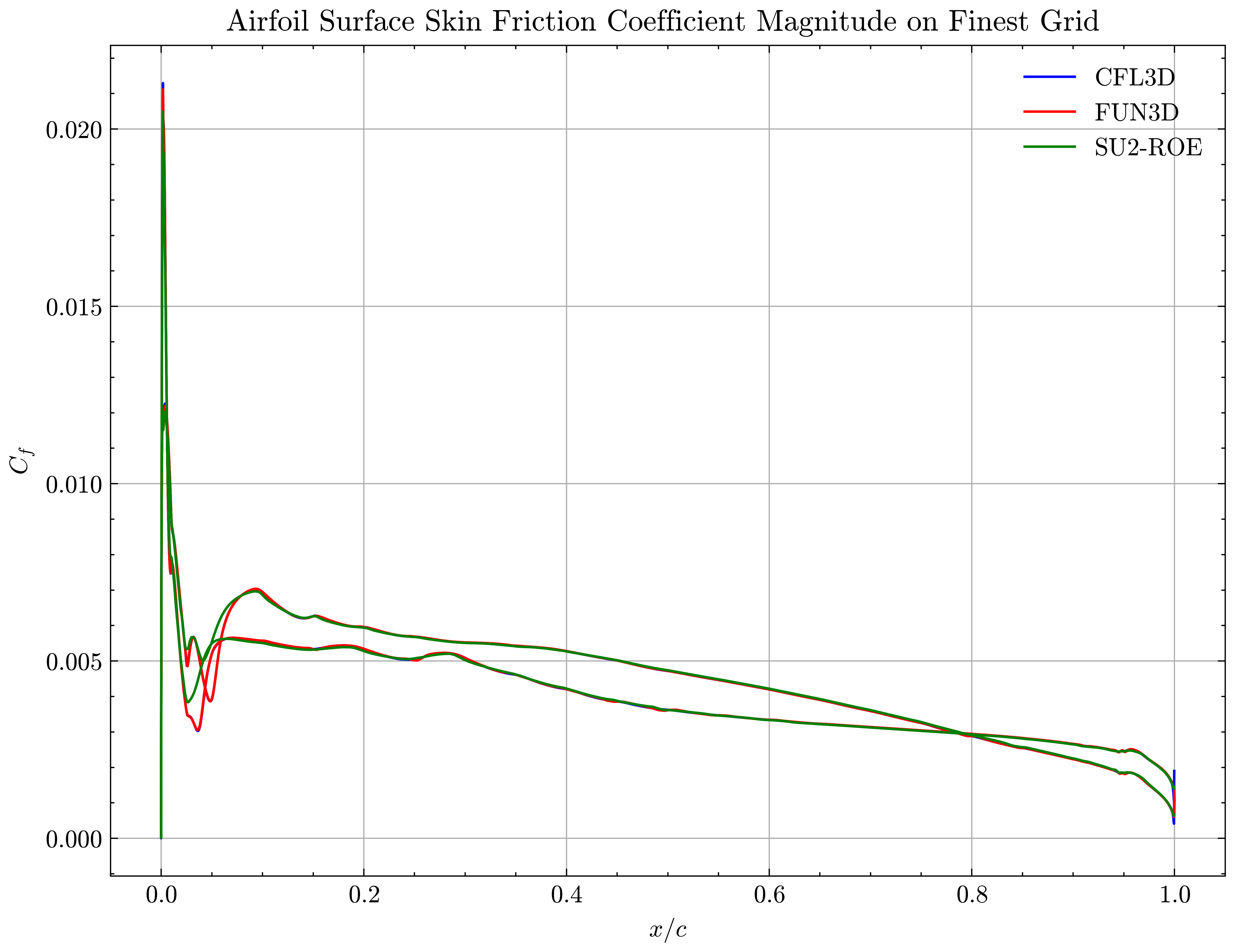
Figure (46): Airfoil Surface Skin Friction Coefficient on Finest Grid