Quick Start

Introduction

Welcome to the Quick Start Tutorial for the SU2 software suite. This tutorial is intended to demonstrate some of the key features of the analysis and design tools in an easily accessible format. Completion of this tutorial only requires a few minutes. If you haven’t done so already, please visit the Download and Installation pages to obtain the most recent stable release of the software and details for installation. This tutorial requires only the SU2_CFD tool from the SU2 suite.

Goals

Upon completing this simple tutorial, the user will be familiar with performing the flow and continuous adjoint simulation of external, inviscid flow around a 2D geometry and be able to plot both the flow solution and the surface sensitivities that result. The specific geometry chosen for the tutorial is the NACA 0012 airfoil. Consequently, the following capabilities of SU2 will be showcased in this tutorial:

• Steady, 2D, Euler and Continuous Adjoint Euler equations
• Multigrid
• JST numerical scheme for spatial discretization
• Euler implicit time integration
• Euler Wall and Farfield boundary conditions

Resources

The files necessary to run this tutorial are included in the SU2/QuickStart/ directory. For the other tutorials, the files will be found in the TestCases/ repository. Two files are needed as input to the code: a configuration file describing the options for the particular problem, and the corresponding computational mesh file. The files are in QuickStart/ and can also be found in the TestCases repository under TestCases/euler/naca0012.

Tutorial

The following tutorial will walk you through the steps required to compute the flow and adjoint solutions around the NACA 0012 airfoil using SU2. Again, we assume that you have already obtained and compiled the SU2_CFD code (either individually, or as part of the complete SU2 package) for a serial computation. If you have yet to complete this requirement, please see the Download and Installation pages.

Background

The NACA0012 airfoil is one of the four-digit wing sections developed by the National Advisory Committee for Aeronautics (NACA), and it is a widely used geometry for many CFD test cases. The numbering system is such that the first number indicates the maximum camber (in percent of chord), the second shows the location of the maximum camber (in tens of percent of chord) and the last two digits indicate the maximum thickness (in percent of chord). More information on these airfoil sections can be found here or in the book ‘Theory of Wing Sections’ by Abbott and von Doenhoff.

Problem Setup

This problem will solve the Euler equations on the NACA0012 airfoil at an angle of attack of 1.25 degrees, using air with the following freestream conditions:

• Pressure = 101,325 Pa
• Temperature = 273.15 K
• Mach number = 0.8

The aim is to find the flow solution and the adjoint solution with respect to an objective function defined as the drag on the airfoil.

Mesh Description

The unstructured mesh provided is in the native .su2 format. It consists of 10,216 triangular cells, 5,233 points, and two boundaries (or “markers”) named airfoil and farfield. The airfoil surface uses a flow-tangency Euler wall boundary condition, while the farfield uses a standard characteristic-based boundary condition. The figure below gives a view of the mesh.

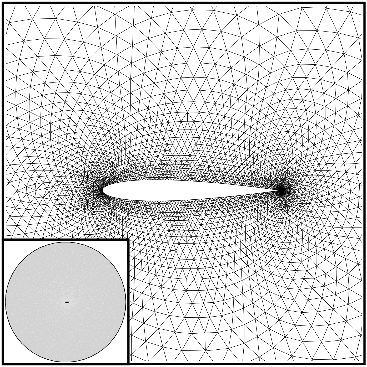
Figure (1): Far-field and zoom view of the computational mesh.

Configuration File Options

Aside from the mesh, the only other file required to run the SU2_CFD solver details the configuration options. It defines the problem, including all options for the numerical methods, flow conditions, multigrid, etc., and also specifies the names of the input mesh and output files. In keeping simplicity for this tutorial, only two configuration options will be discussed. More configuration options will be discussed throughout the remaining tutorials.

Upon opening the inv_NACA0012.cfg file in a text editor, one of the early options is the MATH_PROBLEM:

% Mathematical problem (DIRECT, CONTINUOUS_ADJOINT, DISCRETE_ADJOINT)
MATH_PROBLEM= DIRECT

SU2 is capable of running the direct and adjoint problems for several sets of equations. The direct analysis solves for the flow around the geometry, and quantities of interest such as the lift and drag coefficient on the body will be computed. Solving the adjoint problem leads to an efficient method for obtaining the change in a single objective function (e.g., the drag coefficient) relative to a large number of design variables (surface deformations). The direct and adjoint solutions often couple to provide the objective analysis and gradient information needed by an optimizer when performing aerodynamic shape design. In this tutorial, we will perform DIRECT and CONTINUOUS_ADJOINT solutions for the NACA 0012 airfoil.

The user can also set the format for the solution files:

% Output file format
OUTPUT_FORMAT= TECPLOT

SU2 can output solution files in the .vtk (ParaView), .dat (Tecplot ASCII), and .plt (Tecplot binary) formats which can be opened in the ParaView and Tecplot visualization software packages, respectively. We have set the file type to TECPLOT in this tutorial by default, but users without access to Tecplot are encouraged to download and use the freely available ParaView package. To output solution files for ParaView, set the OUTPUT_FORMAT option to PARAVIEW.

Running SU2

The first step in this tutorial is to solve the Euler equations:

1. Either navigate to the QuickStart/ directory or create a directory in which to run the tutorial. If you have created a new directory, copy the config file (inv_NACA0012.cfg) and the mesh file (mesh_NACA0012_inv.su2) to this directory.
2. Run the executable by entering “SU2_CFD inv_NACA0012.cfg” at the command line. If you have not set the $SU2_RUN environment variable you will need to run “../bin/SU2_CFD inv_NACA0012.cfg” (from the QuickStart directory) or use the appropriate path to your SU2_CFD executable at the command line.
3. SU2 will print residual updates with each iteration of the flow solver, and the simulation will finish after reaching the specified convergence criteria.
4. Files containing the flow results (with “flow” in the file name) will be written upon exiting SU2. The flow solution can be visualized in ParaView (.vtk) or Tecplot (.dat or .plt). More specifically, these files are:
   • flow.dat or flow.vtk - full volume flow solution.
   • surface_flow.dat or surface_flow.vtk - flow solution along the airfoil surface.
   • surface_flow.csv - comma separated values (.csv) file containing values along the airfoil surface.
   • restart_flow.dat - restart file in an internal format for restarting this simulation in SU2.
   • history.dat or history.csv - file containing the convergence history information.

Next, we want to run the adjoint solution to get the sensitivity of the objective function (the drag over the airfoil) to conditions within the flow:

1. Open the config file and change the parameter MATH_PROBLEM from DIRECT to CONTINUOUS_ADJOINT, and save this file.
2. Rename the restart file (restart_flow.dat) to “solution_flow.dat” so that the adjoint code has access to the direct flow solution.
3. Run the executable again by entering “SU2_CFD inv_NACA0012.cfg” at the command line.
4. SU2 will print residual updates with each iteration of the adjoint solver, and the simulation will finish after reaching the specified convergence criteria.
5. Files containing the adjoint results (with “adjoint” in the file name) will be written upon exiting SU2. The flow solution can be visualized in ParaView (.vtk) or Tecplot (.dat or .plt). More specifically, these files are:
   • adjoint.dat or adjoint.vtk - full volume adjoint solution.
   • surface_adjoint.dat or surface_adjoint.vtk - adjoint solution along the airfoil surface.
   • surface_adjoint.csv - comma separated values (.csv) file containing values along the airfoil surface.
   • restart_adj_cd.dat - restart file in an internal format for restarting this simulation in SU2. Note that the name of the objective appears in the file name.
   • history.dat or history.csv - file containing the convergence history information.

Note that as of SU2 v4.1, you can also compute a discrete adjoint for the Euler equations. Assuming that you have built the code with algorithmic differentiation support, you can run the discrete adjoint with the following steps instead:

1. Open the config file and change the parameter MATH_PROBLEM from DIRECT to DISCRETE_ADJOINT, and save this file.
2. Rename the restart file (restart_flow.dat) to “solution_flow.dat” so that the adjoint code has access to the direct flow solution.
3. Run the executable again by entering “SU2_CFD_AD inv_NACA0012.cfg” at the command line. Note that the SU2_CFD_AD executable will only be available when the source has been compiled with AD support.

Results

The following figures were created in Tecplot using the SU2 results. These results are contained in the flow.dat, surface_flow.dat, adjoint.dat, and surface_adjoint.dat files.

Flow Solution

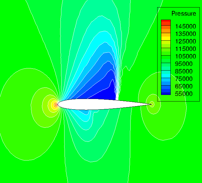
Figure (2): Pressure contours around the NACA 0012 airfoil.

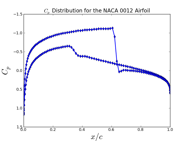
Figure (3): Coefficient of pressure distribution along the airfoil surface. Notice the strong shock on the upper surface (top line) and a weaker shock along the lower surface (bottom line).

Adjoint Solution

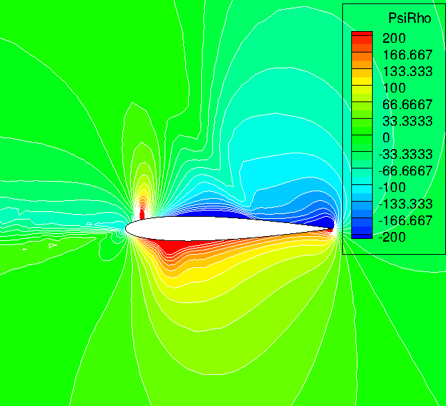
Figure (4): Contours of the adjoint density variable.

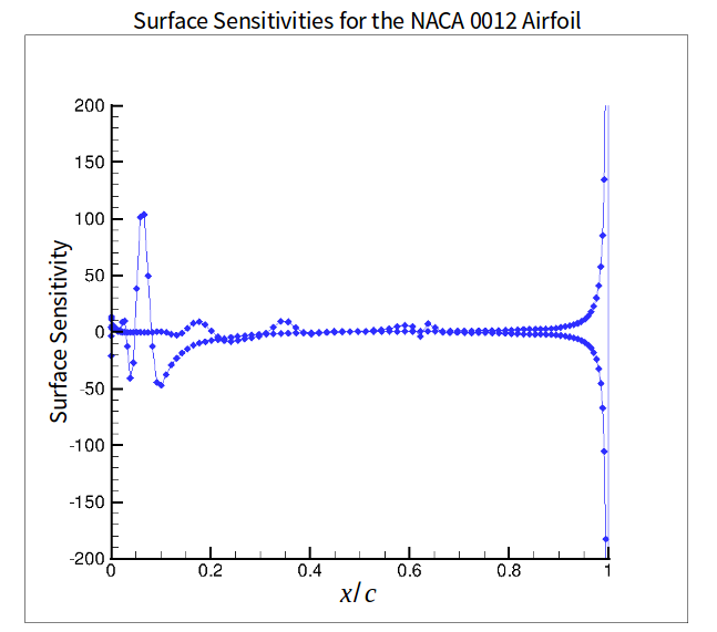
Figure (5): Surface sensitivities. The surface sensitivity is the change in the objective function due to an infinitesimal deformation of the surface in the local normal direction. These values are calculated at each node on the airfoil surface from the flow and adjoint solutions at negligible computational cost using an additional step not described in this tutorial.

Congratulations! You’ve successfully performed your first flow simulations with SU2. Move on to the tutorials to learn much more about using the code, and don’t forget to read through the information in the user’s guide. Having problems with the quick start or visualizing the results? Visit the FAQs page, or see our forum at CFD-online.