-
Inviscid Bump in a Channel
Inviscid Supersonic Wedge
Inviscid ONERA M6
Laminar Flat Plate
Laminar Cylinder
Turbulent Flat Plate
Transitional Flat Plate
Transitional Flat Plate for T3A and T3A-
Turbulent ONERA M6
Unsteady NACA0012
Epistemic Uncertainty Quantification of RANS predictions of NACA 0012 airfoil
Non-ideal compressible flow in a supersonic nozzle
Non-ideal compressible flows with physics-informed neural networks
Aachen turbine stage with Mixing-plane
-
Inviscid Hydrofoil
Laminar Flat Plate with Heat Transfer
Turbulent Flat Plate
Turbulent NACA 0012
Laminar Backward-facing Step
Laminar Buoyancy-driven Cavity
Streamwise Periodic Flow
Species Transport
Composition-Dependent model for Species Transport equations
Unsteady von Karman vortex shedding
Turbulent Bend with wall functions
Wind velocity and pollutant dispersion in a city
-
Static Fluid-Structure Interaction (FSI)
Dynamic Fluid-Structure Interaction (FSI) using the Python wrapper and a Nastran structural model
Static Conjugate Heat Transfer (CHT)
Unsteady Conjugate Heat Transfer
Solid-to-Solid Conjugate Heat Transfer with Contact Resistance
Incompressible, Laminar Combustion Simulation
User Defined combustion model with Python
-
Unconstrained shape design of a transonic inviscid airfoil at a cte. AoA
Constrained shape design of a transonic turbulent airfoil at a cte. CL
Constrained shape design of a transonic inviscid wing at a cte. CL
Shape Design With Multiple Objectives and Penalty Functions
Unsteady Shape Optimization NACA0012
Unconstrained shape design of a two way mixing channel
Adjoint design optimization of a turbulent 3D pipe bend
Actuator Disk With Variable Load
| Written by | for Version | Revised by | Revision date | Revised version |
|---|---|---|---|---|
| @Ettore Saetta, Renato Tognaccini | 7.0.8 | @ |
Solver: |
|
Uses: |
|
Prerequisites: |
None |
Complexity: |
Goals
Upon completing this tutorial, the user will be able to simulate the presence of a propeller by a general actuator disk boundary condition. The model enables the simulation of propellers with variable load distribution and including swirl. The specific geometry chosen for the tutorial is composed by an actuator disk and a semi-infinite spinner (grid file and propeller data courtesy of Mauro Minervino, Centro Italiano Ricerche Aerospaziali (CIRA)).
This tutorial is referred only to the actuator disk model VARIABLE_LOAD implemented in the V7.0.7.
Resources
The resources for this tutorial can be found in the compressible_flow/ActuatorDisk_VariableLoad directory in the Tutorials repository. You will need the configuration file (propeller_variable_load.cfg), the mesh file (propeller_variable_load.su2) and the propeller input data file (ActuatorDisk.dat). It is important to note that the grid used in this tutorial is very coarse to keep computational effort low, finer meshes should be used.
It is also presented the use of OptimalPropeller.py script, very useful tool to generate a propeller input data file with variable load when only total thrust is known.
Tutorial
The following tutorial will walk you through the steps required when solving a flow in presence of a propeller using SU2. The tutorial will also shows how to generate the propeller input data file witht the help of the OptimalPropeller.py script when only total thrust is known. To this end, it is assumed you have already obtained and compiled SU2_CFD. If you have yet to complete these requirements, please see the Download and Installation pages.
Background
This test case is for an actuator disk with a semi-infinite spinner. The actuator disk is a model used to simulate the effects on the aiframe of rotary wings by a simple momentum theory [1]. In aeronautics it is a crucial topic for the airframe integration. Nowadays, a good actuator disk model is getting importance in order to simulate the effects of the propellers of given performance on the airframe by fast CFD analysis. However, the disadvantage of using an actuator disk model is that the unsteady effects are neglected.
The actuator disk model used in this tutorial has been implemented referring to a propeller, so the input data file is suitable for a propeller, but not for a wind turbine. However, the model itself, can also be suitable for any rotary wing device. Note that the model has been tested only for propellers.
The hypothesis that we will consider are: compressible and axial flow (the angle between propeller axis and freestream is small).
Problem Setup
This problem will solve the flow with these conditions:
- Freestream Mach number = 0.55996
- Angle of attack (AOA) = 0.0 deg
- Reynolds number = 3.65E7 (based on propeller diameter)
- Reynolds length = 5.0292 m
The global propeller data are:
- Thrust coefficient = 0.15
- Advance Ratio = 2.81487
- Radius = 2.5146 m
The thrust coefficient is defined using the “Renard” definition: the reference force is \(\rho n^2D^4\), where n are the propeller rounds per second and D is the propeller diameter The advance ratio is defined as \(J=\frac{V_\infty}{nD}\).
Mesh Description
The computational domain contains the actuator disk mounted on a semi-infinite spinner. The mesh consists of 48,736 elements and 51,847 nodes. Again, we note that this is a very coarse mesh, and should one wish to obtain more accurate solutions for comparison with results in the literature, finer grids should be used.
Three boundary conditions are employed:
- Actuator Disk on the two surfaces (upstream and downstream) of the actuator disk.
- Navier-Stokes adiabatic wall on the spinner.
- Far-field condition on the outer domain surface.
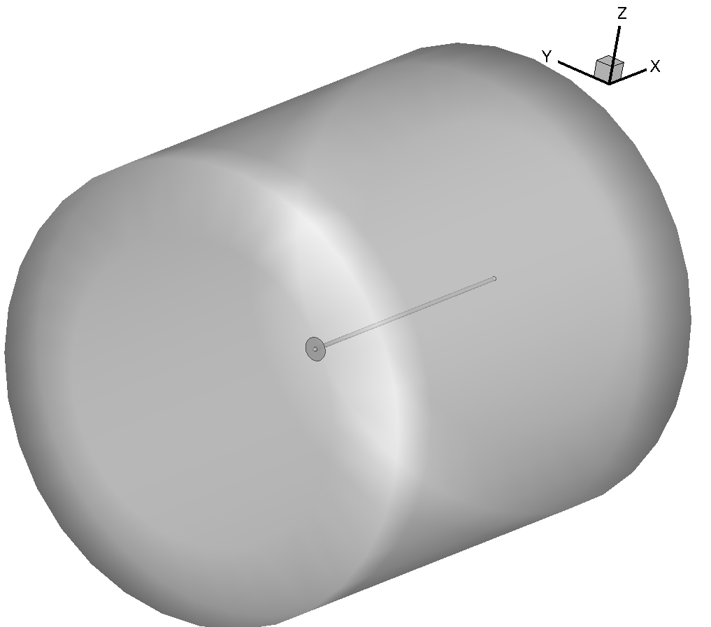 Figure (1): Far-field view of the computational domain.
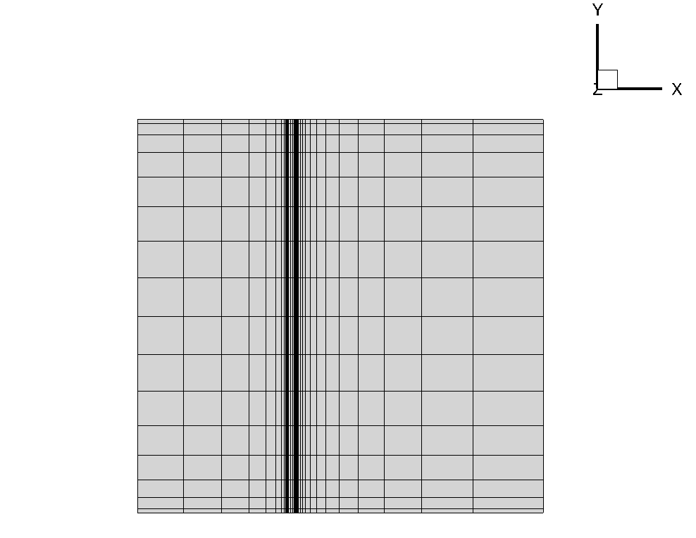 Figure (2): Mesh of the domain in the x-y plane.
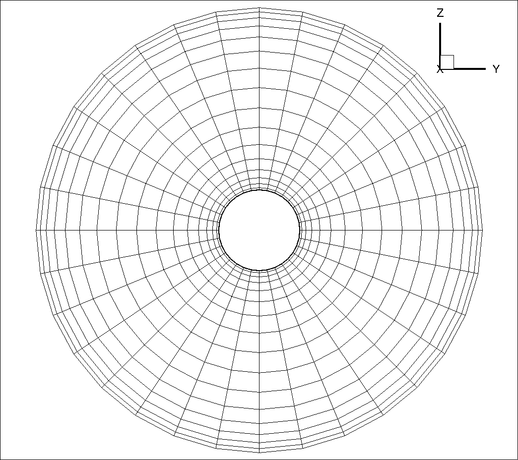 Figure (3): Close-up view of the mesh of the actuator disk in the y-z plane at x=0.
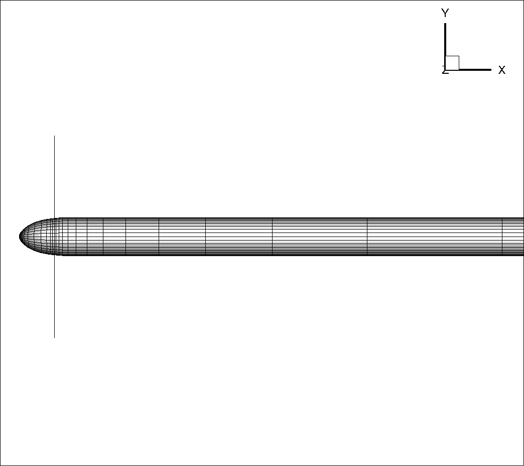 Figure (4): Close-up view of the mesh of the spinner in the y-x plane.
Configuration File Options
Only the actuator disk boundary condition options are highlighted here:
% -------------------- ACTUATOR DISK BOUNDARY CONDITION --------------------------%
%
ACTDISK_DOUBLE_SURFACE = YES
%
% Actuator disk boundary type (VARIABLE_LOAD, VARIABLES_JUMP, BC_THRUST,
%                              DRAG_MINUS_THRUST)
ACTDISK_TYPE= VARIABLE_LOAD
%
% Actuator disk data input file name
ACTDISK_FILENAME= ActuatorDisk.dat
%
% Actuator disk boundary marker(s) with the following formats (NONE = no marker)
% Variable Load: (inlet face marker, outlet face marker,
%                 0.0, 0.0, 0.0, 0.0, 0.0, 0.0) Markers only effectively used.
MARKER_ACTDISK = ( DISK, DISK_BACK, 0.0, 0.0, 0.0, 0.0, 0.0, 0.0 )
The ACTDISK_DOUBLE_SURFACE option, in this case, is set to true because the actuator disk surface has been splitted in two parts: upstream and sownstream surfaces.
The ACTDISK_TYPE option, is used to choose the actuator disk boundary type. In this tutorial, we consider a variable load distribution along the disk, and that also take the swirl term into consideration. The actuator disk type that meets these conditions is the VARIABLE_LOAD.
The ACTDISK_FILENAME option is used to specify the name of the actuator disk data input file. Further we will see how to generate this file if only total thrust is known and not the details on the load distribution.
The MARKER_ACTDISK option, requires the following arguments:
- Marker of the upstream surface of the actuator disk.
- Marker of the downstream surface of the actuator disk.
- 6 zero arguments. These arguments have a different meaning using different
ACTDISK_TYPE. In this case, they are all set to0.0because they are not needed.
If there are more actuator disks, it is possible to append them in the MARKER_ACTDISK option.
Input Data File
The input data file is needed for the VARIABLE_LOAD actuator disk type.
An example of this file (used in this tutoral) is here reported:
MARKER_ACTDISK= DISK DISK_BACK
CENTER= 0.0 0.0 0.0
AXIS= 1.0 0.0 0.0
RADIUS= 2.5146
ADV_RATIO= 2.81487
NROW= 37
# rs=r/R    dCT/drs     dCP/drs     dCR/drs
  0.2031   0.020066   0.0890674         0.0
  0.2235   0.019963   0.0932674         0.0
  0.2439   0.021707   0.0982980         0.0
  0.2644   0.024667   0.1064153         0.0
  0.2848   0.029147   0.1189045         0.0
  0.3257   0.043674   0.1588513         0.0
  0.3461   0.053380   0.1849900         0.0
  0.3665   0.064327   0.2145367         0.0
  0.3870   0.076521   0.2471873         0.0
  0.4278   0.103679   0.3203392         0.0
  0.4483   0.118918   0.3609085         0.0
  0.4687   0.135619   0.4051864         0.0
  0.4891   0.152986   0.4518863         0.0
  0.5096   0.171453   0.5011266         0.0
  0.5300   0.190755   0.5528521         0.0
  0.5504   0.211062   0.6072281         0.0
  0.5709   0.231313   0.6620508         0.0
  0.5913   0.251252   0.7161404         0.0
  0.6117   0.271376   0.7700722         0.0
  0.6322   0.290980   0.8219708         0.0
  0.6526   0.309848   0.8715231         0.0
  0.6730   0.328502   0.9202496         0.0
  0.6935   0.346774   0.9681596         0.0
  0.7139   0.364895   1.0156277         0.0
  0.7343   0.381991   1.0603740         0.0
  0.7548   0.398417   1.1036331         0.0
  0.7752   0.413550   1.1442054         0.0
  0.7956   0.427447   1.1820164         0.0
  0.8161   0.440093   1.2163819         0.0
  0.8365   0.451007   1.2453084         0.0
  0.8569   0.460535   1.2682212         0.0
  0.8774   0.467765   1.2823500         0.0
  0.8978   0.471296   1.2839416         0.0
  0.9182   0.470303   1.2701343         0.0
  0.9387   0.460921   1.2317719         0.0
  0.9591   0.434937   1.1470356         0.0
  0.9795   0.377288   0.9746048         0.0
The MARKER_ACTDISK option, as the same for the configuration file, is used to specify the markers of the actuator disk surfaces. All the next propeller data will be referred to these surfaces.
The CENTER option contains the coordinates of the actuator disk center, expressed in the grid reference system.
The AXIS option contains the components of the unit vector normal to the actuator disk surface.
The RADIUS option is used to specify the actuator disk radius.
The ADV_RATIO option contains the advance ratio of the propeller defined as \(J=\frac{V_\infty}{nD}\), where n are the propeller rounds per second and D is the propeller diameter.
The NROW option isused to indicate the number of radial stations of the actuator disk in which we assign the load distribution.
The next row is a dummy row, so it is skipped.
Then there are 4 columns containing respectively:
- The non dimensional radial station $$\overline{r}=\frac{r}{R}$
- The thrust coefficient distribution \(\frac{\mathrm{d}C_T}{\mathrm{d}\overline{r}}\)
- The power coefficient distribution $$\frac{\mathrm{d}C_P}{\mathrm{d}\overline{r}}$
- The radial force coefficient distribution \(\frac{\mathrm{d}C_R}{\mathrm{d}\overline{r}}\)
These coefficients are defined using the “Renard” definition: the reference force is \(\rho n^2D^4\), while the reference power is reference force is \(\rho n^3D^5\)
It is possible to append other propellers data at the end of the input file. Note that the order and the format of the options should not be changed.
The visualization of the tabular input for this case is shown in the following figure:
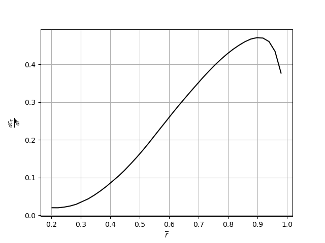 Figure (5): Thrust coefficient distribution along the non-dimensional radius.
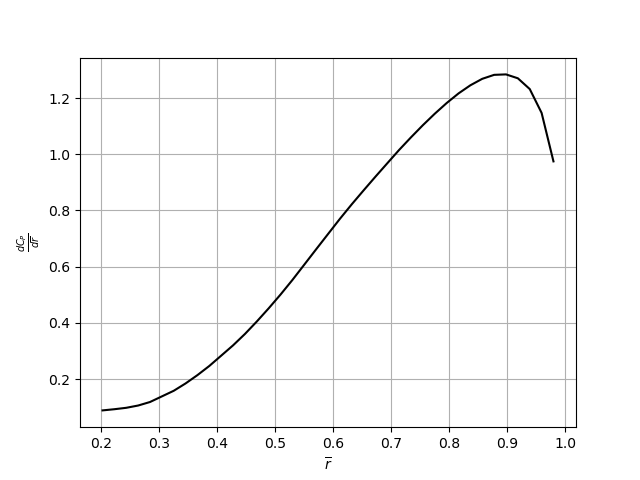 Figure (6): Power coefficient distribution along the non-dimensional radius.
Optimal Propeller Script
As already anticipated, the OptimalPropeller.py script can be used to automatically generate the propeller input data file when the details on the variable load are not known.
This script allows the user to use the VARIABLE_LOAD actuator disk type also when only total thrust is known. The variable load distribution is obtained by the inviscid theory of the optimal propeller [1].
The input is interactive, and requires the following data:
- Number of radial stations (where local data should be generated).
- \(CT\): the total thrust coefficient defined using the “Renard” definition.
- \(R\): The propeller radius expressed in meters.
- \(r_{\textrm{hub}}\): the hub radius expressed in meters.
- \(J\): the advance ratio.
- \(V_{\textrm{inf}}\): the free-stream velocity expressed in m/s.
- Here, the script asks if you want to use the tip loss Prandtl correction (yes is the default choise).
- \(N\): if you chose yes in the previous stage, it requires also the number of propeller blades.
Once the input is given, the script provides 3 plots showing the tip loss Prandtl correction function, the axial and rotational interference factors and the thrust and power coefficients distributions along the non dimentional radius. The script also provides 2 files:
- ActuatorDisk.cfg: containing the actuator disk boundary condition options needed in the configuration file.
- ActuatorDisk.dat: containing the propeller input data file.
Note that the two generated files have some empty fields that need to be filled.
References
[1] Glauert H., Airplane Propellers, in Aerodynamic Theory, Ed. Durand W. F., Vol. IV, pp. 169 - 360, Springer, 1935.
Running SU2
The actuator disk with variable load test case is small and will execute relatively quickly on a single workstation or laptop in serial. To run this test case, follow these steps at a terminal command line:
- Move to the directory containing the configuration file (propeller_variable_load.cfg), the mesh file (propeller_variable_load.su2) and the propeller input data file (ActuatorDisk.dat). Make sure that the SU2 tools were compiled, installed, and that their install location was added to your path.
-
Run the executable by entering
$ SU2_CFD propeller_variable_load.cfgat the command line.
- SU2 will print residual updates with each iteration of the flow solver, and the simulation will terminate after meeting the specified convergence criteria.
- Files containing the results will be written upon exiting SU2. The flow solution can be visualized in ParaView (.vtk) or Tecplot (.dat for ASCII).
Results
Some results for this test case are shown below.
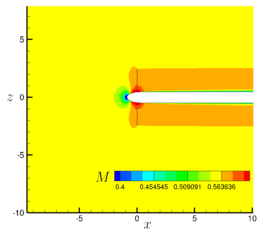 Figure (7): Mach number contour in the x-z plane.
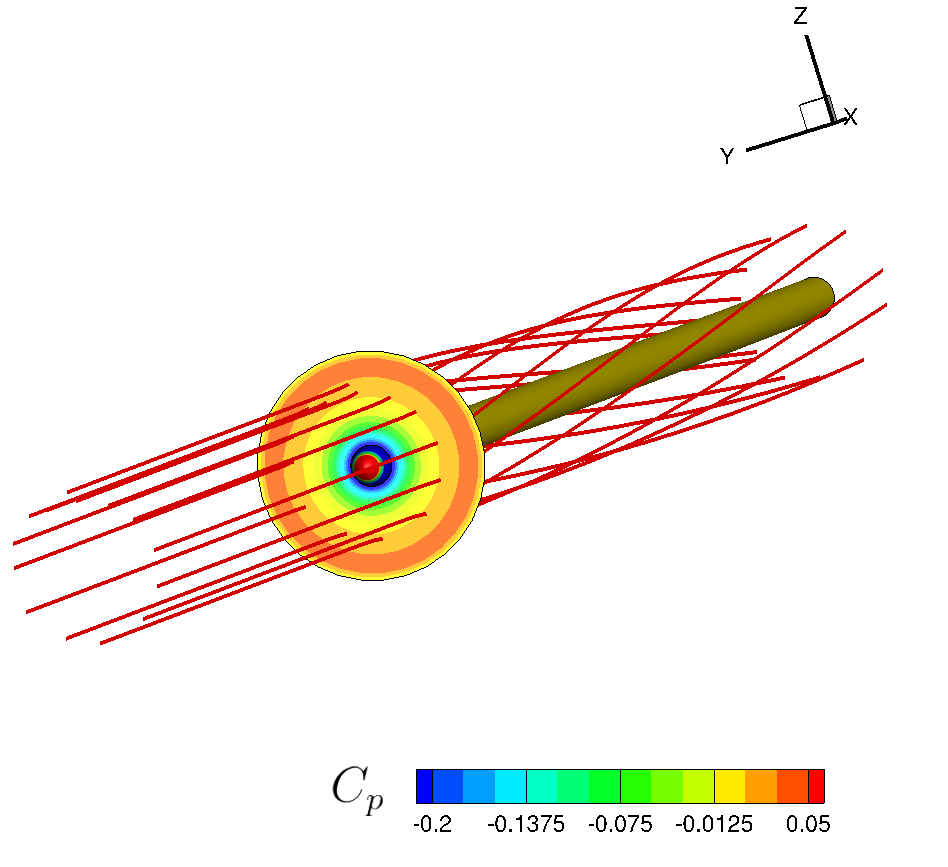
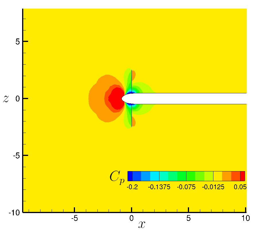 Figure (8): Pressure coefficient contour in the x-z plane.
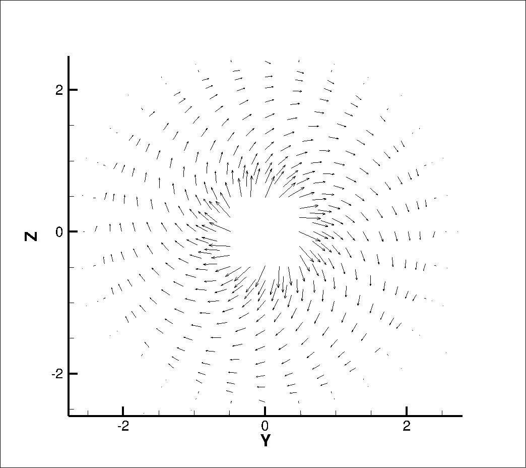 Figure (9): Tangential velocity vectors just downstream the actuator disk. Swirl effect visualization.
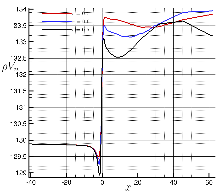 Figure (10): Momentum in normal direction along x for different stations.
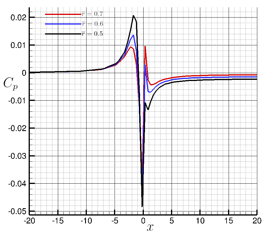 Figure (11): Pressure coefficient along x for different stations.
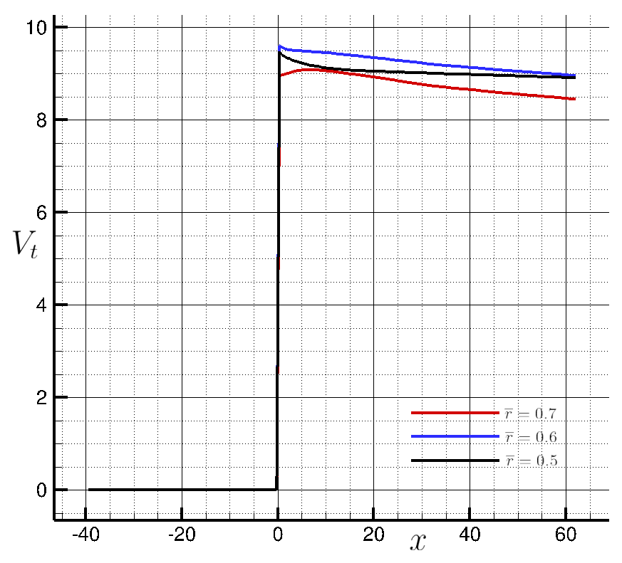 Figure (12): Tangential velocity component along x for different stations.
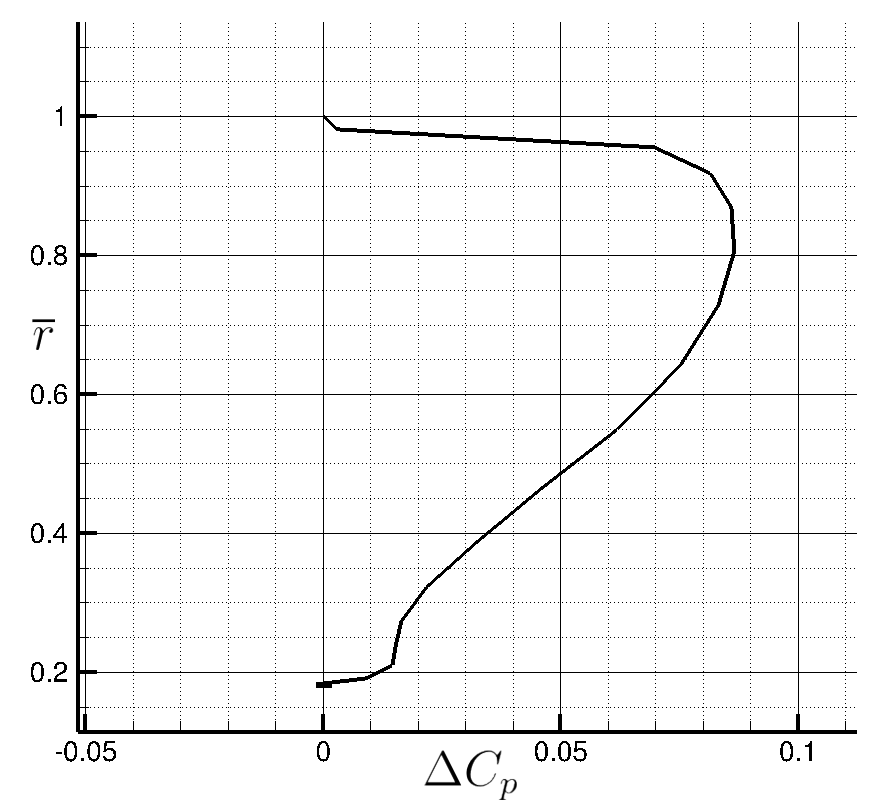 Figure (13): Pressure coefficient jump along the non-dimensional radius.
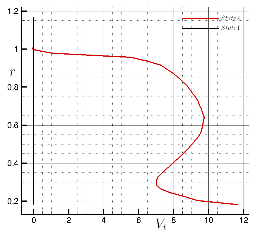 Figure (14): Tangential velocity component along z just upstream (State 1) and downstream (State 2) the actuator disk.