Laminar Flat Plate

Goals

Upon completing this tutorial, the user will be familiar with performing a simulation of external, laminar flow over a flat plate. The solution will provide a laminar boundary layer on the surface, which can be compared to the Blasius solution as a verification case for SU2. Consequently, the following capabilities of SU2 will be showcased in this tutorial:

• Steady, 2D, Laminar Navier-Stokes equations
• Multigrid
• Roe convective scheme in space (2nd-order, upwind)
• Corrected average-of-gradients viscous scheme
• Euler implicit time integration
• Inlet, Outlet, Symmetry, and Navier-Stokes Wall boundary conditions
• Cauchy convergence criteria

The intent of this tutorial is to introduce a common viscous test case which is used to explain the basics of setting up a viscous case in SU2.

Resources

The resources for this tutorial can be found in the compressible_flow/Laminar_Flat_Plate directory in the tutorial repository. You will need the configuration file (lam_flatplate.cfg) and the mesh file (mesh_flatplate_65x65.su2).

Tutorial

The following tutorial will walk you through the steps required when solving for the flow over a flat plate using SU2. It is assumed you have already obtained and compiled the SU2_CFD code for a serial computation. If you have yet to complete these requirements, please see the Download and Installation pages.

Background

In his PhD dissertation in 1908, H. Blasius obtained what is now referred to as the Blasius equation for incompressible, laminar flow over a flat plate:

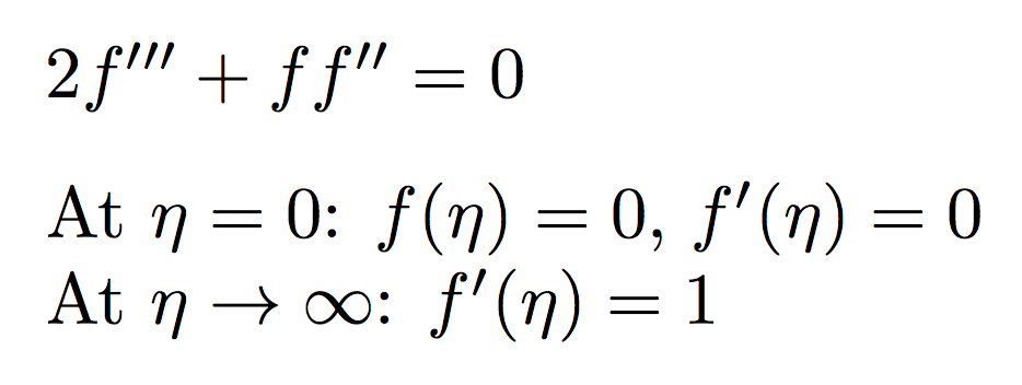
The third-order, ordinary differential equation can be solved numerically using a shooting method resulting in the well-known laminar boundary layer profile. Using the numerical solution, an expression for the skin friction coefficient along the flat plate can also be derived:

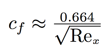
where Re_x is the Reynolds number along the plate. In this tutorial, we will perform a solution of nearly incompressible (low Mach number) laminar flow over a flat plate and compare our results against the analytical Blasius solutions for the profile shape and skin friction coefficient along the plate. This problem has become a classic test case for viscous flow solvers. More detail on the Blasius solution and the similarity variables can be found in Chapter 18 of Fundamentals of Aerodynamics (Fourth Edition) by John D. Anderson, Jr. and most other texts on aerodynamics.

Problem Setup

This problem will solve the for the flow over the flat plate with these conditions:

• Inlet Stagnation Temperature = 300.0 K
• Inlet Stagnation Pressure = 100000.0 N/m2
• Inlet Flow Direction, unit vector (x,y,z) = (1.0, 0.0, 0.0)
• Outlet Static Pressure = 97250.0 N/m2
• Resulting free-stream Mach number = 0.2
• Reynolds number = 1301233.166 for a plate length of 0.3048 m (1 ft)

Mesh Description

The computational mesh for the flat plate is composed of quadrilaterals with 65 nodes in both the x- and y-directions. The flat plate is along the lower boundary of the domain (y = 0) starting at x = 0 m and is of length 0.3048 m (1 ft). In the figure of the mesh, this corresponds to the Navier-Stokes (no-slip) boundary condition highlighted in green. The domain extends a distance upstream of the flat plate, and a symmetry boundary condition is used to simulate a free-stream approaching the plate in this region (highlighted in purple). Axial stretching of the mesh is used to aid in resolving the region near the start of the plate where the no-slip boundary condition begins at x = 0 m, as shown in Figure (1).

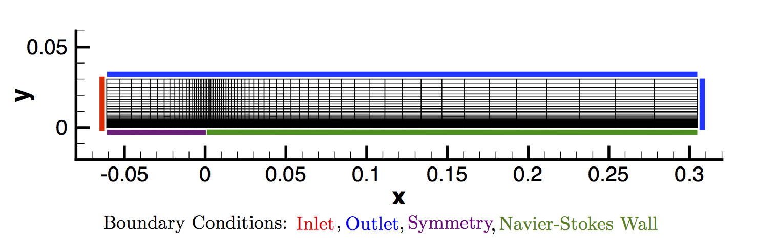Figure (1): Figure of the computational mesh with boundary conditions.

Because the flow is subsonic and disturbances caused by the presence of the plate can propagate both upstream and downstream, characteristic-based, subsonic inlet and outlet boundary conditions are used for the flow entrance plane (red) and the outflow regions along the upper region of the domain and the exit plane at x = 0.3048 m (blue).

In any simulation of viscous flow, it is important to capture the behavior of the boundary layer. Doing so requires an appropriate level of grid refinement near the wall. In this mesh, the vertical spacing is such that approximately 30 grid nodes lie within the boundary layer, which is typical for laminar flows of this nature.

Configuration File Options

Several of the key configuration file options for this simulation are highlighted here. As this is our first viscous problem in the tutorials, we set the problem definition for a viscous flow:

% ------------- DIRECT, ADJOINT, AND LINEARIZED PROBLEM DEFINITION ------------%
%
% Physical governing equations (EULER, NAVIER_STOKES,
%                               WAVE_EQUATION, HEAT_EQUATION, FEM_ELASTICITY,
%                               POISSON_EQUATION)
SOLVER= NAVIER_STOKES
%
% Specify turbulence model (NONE, SA, SA_NEG, SST)
KIND_TURB_MODEL= NONE

To compute viscous flows, the Navier-Stokes governing equations are selected. The option NAVIER_STOKES implies that we wish to solve a laminar Navier-Stokes problem, and therefore, we must also set KIND_TURB_MODEL= NONE. For turbulent flows, SU2 solves the Reynolds-averaged Navier-Stokes equations by setting SOLVER= RANS, and SU2 currently contains implementations of the Spalart-Allmaras model and several variants (SA, SA_NEG, etc.) and the Shear Stress Transport (SST) model of Menter. If this were an inviscid flow problem, the user would enter SOLVER = EULER for the problem type. SU2 supports other governing equations, as well, and the user is invited to review the governing equations documentation page for a description of the possible options.

Defining a no-slip boundary condition for viscous walls can be accomplished in one of two ways:

% -------------------- BOUNDARY CONDITION DEFINITION --------------------------%
%
% Navier-Stokes (no-slip), constant heat flux wall  marker(s) (NONE = no marker)
% Format: ( marker name, constant heat flux (J/m^2), ... )
MARKER_HEATFLUX= ( wall, 0.0 )
%
% Navier-Stokes (no-slip), isothermal wall marker(s) (NONE = no marker)
% Format: ( marker name, constant wall temperature (K), ... )
MARKER_ISOTHERMAL= ( NONE )

An adiabatic, no-slip boundary condition can be selected by using the MARKER_HEATFLUX option with the value of the heat flux set to 0.0. An isothermal wall condition is also available with a similar format for setting a fixed temperature on the wall.

The convective fluxes are computed with a 2nd-order upwind method, and the viscous terms are computed with the corrected average-of-gradients method (the default in SU2). We will discuss the various options for specifying the convective scheme in the next tutorial. The flow variable gradients needed for the convective and viscous fluxes are calculated via a weighted least squares method, but a Green-Gauss method is also available:

% Numerical method for spatial gradients (GREEN_GAUSS, WEIGHTED_LEAST_SQUARES)
NUM_METHOD_GRAD= WEIGHTED_LEAST_SQUARES

For this problem, we are choosing a typical set of numerical methods. However, it is always advised that users should experiment with various numerical methods for their own problems.

Running SU2

The flat plate simulation for the 65x65 node mesh is small and will execute relatively quickly on a single workstation or laptop in serial. To run this test case, follow these steps at a terminal command line:

1. Move to the directory containing the config file (lam_flatplate.cfg) and the mesh file (mesh_flatplate_65x65.su2). Make sure that the SU2 tools were compiled, installed, and that their install location was added to your path.

2. Run the executable by entering

   $ SU2_CFD lam_flatplate.cfg
   

   at the command line.

3. SU2 will print residual updates with each iteration of the flow solver, and the simulation will terminate after reaching the specified convergence criteria.
4. Files containing the results will be written upon exiting SU2. The flow solution can be visualized in ParaView (.vtk) or Tecplot (.dat for ASCII).

Results

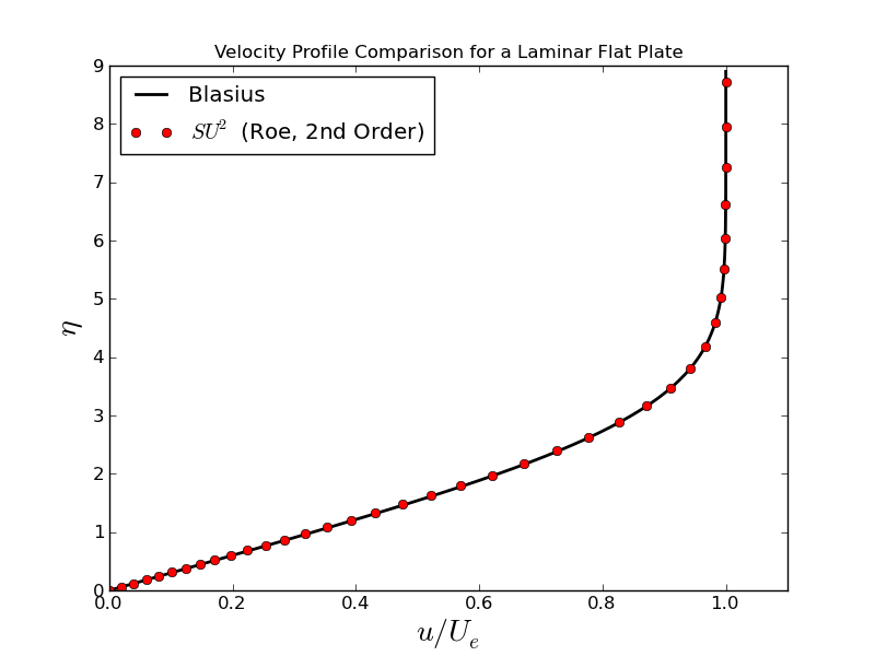
Results are given here for the SU2 solution of laminar flow over the flat plate. The results show excellent agreement with the closed-form Blasius solution.

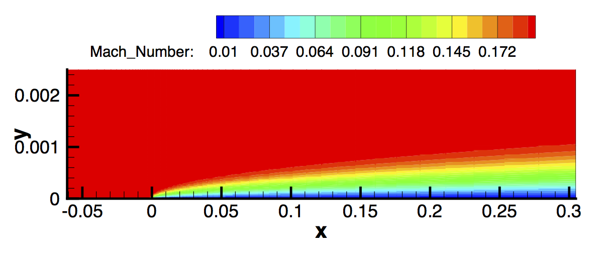Figure (2): Mach contours for the laminar flat plate.

Figure (3): Velocity data was extracted from the exit plane of the mesh (x = 0.3048 m) near the wall, and the boundary layer velocity profile was plotted compared to and using the similarity variables from the Blasius solution.

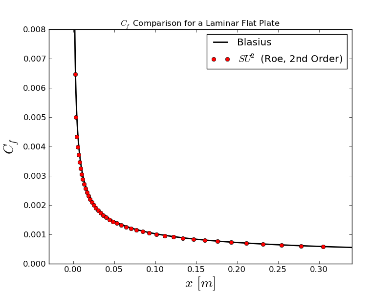Figure (4): A plot of the skin friction coefficient along the plate created using the values written in the surface_flow.csv file and compared to Blasius.