-
Inviscid Bump in a Channel
Inviscid Supersonic Wedge
Inviscid ONERA M6
Laminar Flat Plate
Laminar Cylinder
Turbulent Flat Plate
Transitional Flat Plate
Transitional Flat Plate for T3A and T3A-
Turbulent ONERA M6
Unsteady NACA0012
Epistemic Uncertainty Quantification of RANS predictions of NACA 0012 airfoil
Non-ideal compressible flow in a supersonic nozzle
Non-ideal compressible flows with physics-informed neural networks
Aachen turbine stage with Mixing-plane
-
Inviscid Hydrofoil
Laminar Flat Plate with Heat Transfer
Turbulent Flat Plate
Turbulent NACA 0012
Laminar Backward-facing Step
Laminar Buoyancy-driven Cavity
Streamwise Periodic Flow
Species Transport
Composition-Dependent model for Species Transport equations
Unsteady von Karman vortex shedding
Turbulent Bend with wall functions
Wind velocity and pollutant dispersion in a city
-
Static Fluid-Structure Interaction (FSI)
Dynamic Fluid-Structure Interaction (FSI) using the Python wrapper and a Nastran structural model
Static Conjugate Heat Transfer (CHT)
Unsteady Conjugate Heat Transfer
Solid-to-Solid Conjugate Heat Transfer with Contact Resistance
Incompressible, Laminar Combustion Simulation
User Defined combustion model with Python
-
Unconstrained shape design of a transonic inviscid airfoil at a cte. AoA
Constrained shape design of a transonic turbulent airfoil at a cte. CL
Constrained shape design of a transonic inviscid wing at a cte. CL
Shape Design With Multiple Objectives and Penalty Functions
Unsteady Shape Optimization NACA0012
Unconstrained shape design of a two way mixing channel
Adjoint design optimization of a turbulent 3D pipe bend
Static Fluid-Structure Interaction (FSI)
| Written by | for Version | Revised by | Revision date | Revised version |
|---|---|---|---|---|
| @rsanfer | 7.0.2 | @rsanfer | 2020-02-05 | 7.0.2 |
Solver: |
|
Uses: |
|
User Guide: |
Basics of Multi-Zone Computations |
Prerequisites: |
Non-linear Elasticity |
| |
Inviscid Hydrofoil |
Complexity: |
Intermediate |
Goals
This tutorial combines SU2’s fluid and structural capabilities to solver a steady-state Fluid-Structure Interaction problem. This document will cover:
- Setting up a multiphysics problem in SU2
- Nonlinear structural mechanics and incompressible Navier-Stokes flow
- Coupling boundary conditions on primary config file
- Changes required to the config files of each subproblem
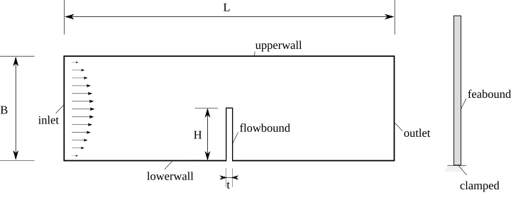
In this tutorial, we use the same problem definition as for most structural tutorials, a vertical, slender cantilever, clamped in its base, but in this case it is immersed in a horizontal flow in a channel. This is shown next:
Resources
You can find the resources for this tutorial in the folder fsi/steady_state of the Tutorials repository. There is a FSI config file and two sub-config files for the flow and structural subproblems.
Moreover, you will need two mesh files for the flow domain and the cantilever.
Background
The equations presented here are a summary of the approach to FSI in SU2 that is further described in R. Sanchez PhD thesis\(^1\). Please refer to this document for more information.
SU2 adopts a partitioned approach for Fluid-Structure Interaction that requires imposing compatibility and continuity conditions at the FSI interface \(\Gamma = \Omega_f \cap \Omega_s\). Continuity of displacements is defined as
\[\mathbf{u}_\Gamma = \mathbf{z}_\Gamma,\]while the equilibrium of tractions over the interface requires that
\[\boldsymbol{\lambda}_f + \boldsymbol{\lambda}_s = 0,\]where \(\boldsymbol{\lambda}_f\) and \(\boldsymbol{\lambda}_s\) are, respectively, the tractions over the fluid and structural sides of \(\Gamma\). They may be defined as
\[\begin{cases} \begin{array}{ll} \boldsymbol{\lambda}_{f} = -p\mathbf{n}_{f}+\boldsymbol{\tau}_{f} \mathbf{n}_{f} &\text{on } \Gamma_{f}, \\ \boldsymbol{\lambda}_{s} = \mathbf{\sigma}_{s} \mathbf{n}_{s} &\text{on } \Gamma_{s}, \\ \end{array} \end{cases}\]where \(\mathbf{n}_{f}\) and \(\mathbf{n}_{s}\) are the dimensional, outward normals to the fluid and structural sides of \(\Gamma\) (including area information).
We define the structural, fluid mesh and fluid problems respectively as \(\mathscr{S}\), \(\mathscr{M}\) and \(\mathscr{F}\). We can write the governing equations of the coupled FSI problem as a function of the problem state variables, \(\mathbf{u}\), \(\mathbf{w}\) and \(\mathbf{z}\), which are respectively the structural displacements, the flow conservative variables and the flow mesh displacements, as
\[\mathscr{G}(\mathbf{u}, \mathbf{w}, \mathbf{z}) = \begin{cases} \renewcommand\arraystretch{1.4} \mathscr{S}(\mathbf{u}, \mathbf{w}, \mathbf{z}) = \mathbf{T}(\mathbf{u}) - \mathbf{F}_b - \mathbf{F}_{\Gamma}(\mathbf{u}, \mathbf{w}, \mathbf{z}) + \rho_s \mathbf{\ddot{u}} = \mathbf{0}, \\ \mathscr{F}(\mathbf{w}, \mathbf{z}) = \mathbf{\dot{w}} + \nabla \cdot \mathbf{F^{c}}(\mathbf{w}, \mathbf{z}, \mathbf{\dot{z}}) - \nabla \cdot \mathbf{F^{v}}(\mathbf{w}, \mathbf{z}) = \mathbf{0}, \\ \mathscr{M}(\mathbf{u}, \mathbf{z}) = \mathbf{\tilde{K}}_{\mathscr{M}}\mathbf{z} - \mathbf{\tilde{f}}(\mathbf{u}) = \mathbf{0}. \end{cases}\]Due to the non-linear nature of the coupled problem, one can apply Newton-Raphson methods to obtain the coupled solution \(^2\). The problem may be linearised within a time step writing it in the form of a Newton iteration
\[\left\{ \begin{array}{ccc} \frac{\partial \mathscr{S}}{\partial \mathbf{u}} & \frac{\partial \mathscr{S}}{\partial \mathbf{w}} & \frac{\partial \mathscr{S}}{\partial \mathbf{z}} \\ \mathbf{0} & \frac{\partial \mathscr{F}}{\partial \mathbf{w}} & \frac{\partial \mathscr{F}}{\partial \mathbf{z}} \\ \frac{\partial \mathscr{M}}{\partial \mathbf{u}} & \mathbf{0} & \frac{\partial \mathscr{M}}{\partial \mathbf{z}} \\ \end{array} \right\} \normalsize \left\{ \begin{array}{cc|cc} \Delta \mathbf{u} \\ \Delta \mathbf{w} \\ \Delta \mathbf{z} \\ \end{array} \right\} = - \left\{ \begin{array}{cc|cc} \mathscr{S}(\mathbf{u}, \mathbf{w}, \mathbf{z}) \\ \mathscr{F}(\mathbf{w}, \mathbf{z}) \\ \mathscr{M}(\mathbf{u}, \mathbf{z}) \\ \end{array} \right\} .\]However, the construction of the previous Jacobian of the problem is complex. In SU2, we avoid it by adopting a Block-Gauss-Seidel (BGS) strategy, which allows the sequential solution of the three problems within each FSI iteration,
\[\left\{ \begin{array} {ccc} \frac{\partial \mathscr{S}}{\partial \mathbf{u}} & 0 & 0 \\ 0 & \frac{\partial \mathscr{F}}{\partial \mathbf{w}} & 0 \\ \frac{\partial \mathscr{M}}{\partial \mathbf{u}} & 0 & \frac{\partial \mathscr{M}}{\partial \mathbf{z}} \end{array} \right\} \left\{ \begin{array}{c} \Delta \mathbf{u} \\ \Delta \mathbf{w} \\ \Delta \mathbf{z} \end{array} \right\} = - \left\{ \begin{array}{c} \mathscr{S}(\mathbf{u},\mathbf{w},\mathbf{z}) \\ \mathscr{F}(\mathbf{w},\mathbf{z}) \\ \mathscr{M}(\mathbf{u},\mathbf{z}) \end{array} \right\}\]The linearized problem in BGS form is solved iteratively until convergence.
Mesh Description
The cantilever is discretized using 1000 4-node quad elements with linear interpolation. The fluid domain is discretized using a finite volume mesh with 7912 nodes and 15292 triangular volumes. The wet interface is matching between the fluid and structural domains.
Configuration File Options
We start the tutorial by definining the problem as a multiphysics case,
SOLVER = MULTIPHYSICS
We set the config files for each sub-problem using the command CONFIG_LIST, and state that each sub-problem will use a different mesh file:
CONFIG_LIST = (config_channel.cfg, config_cantilever.cfg)
MULTIZONE_MESH = NO
Now, we define the outer iteration strategy to solve the FSI problem. We use a Block Gauss-Seidel iteration as defined in the background section with a maximum of 40 outer iterations
MULTIZONE_SOLVER = BLOCK_GAUSS_SEIDEL
OUTER_ITER = 40
Then, the convergence criteria is set to evaluate the averaged residual of the flow state vector (zone 0) (AVG_BGS_RES[0]) and the structural state vector (zone 1) (AVG_BGS_RES[1]) in two consecutive outer iterations, \(\mathbf{w}^{n+1}-\mathbf{w}^{n}\) and \(\mathbf{u}^{n+1}-\mathbf{u}^{n}\) respectively.
CONV_FIELD = AVG_BGS_RES[0], AVG_BGS_RES[1]
CONV_RESIDUAL_MINVAL = -9
Finally, we define the coupling conditions. In this case, the interface between the marker flowbound in the flow field, and feabound in the structural field, is defined as
MARKER_ZONE_INTERFACE = (flowbound, feabound)
The last step is defining our desired output. In this tutorial, we will use the following configuration for the screen output
SCREEN_OUTPUT = (OUTER_ITER, AVG_BGS_RES[0], AVG_BGS_RES[1], DEFORM_MIN_VOLUME[0], DEFORM_ITER[0])
WRT_ZONE_CONV = NO
where the convergence magnitudes are plotted alongside the minimum volume obtained in the deformed mesh, and the number of iterations required by the linear solver that updates the mesh deformation. For clarity, the command WRT_ZONE_CONV limits the output to the outer iterations, while the convergence of the flow and structural sub-problems is not written to screen.
The convergence output will be set using
HISTORY_OUTPUT = ITER, BGS_RES[0], AERO_COEFF[0], BGS_RES[1]

WRT_ZONE_HIST = NO
CONV_FILENAME= history
where the individual components of the flow and structural outer-iteration residuals will be written, together with the convergence of the aerodynamic coefficients for the flow domain. In terms of result output, we use
OUTPUT_FILES = (RESTART, PARAVIEW)
RESTART_FILENAME = restart_fsi_steady
VOLUME_FILENAME = fsi_steady
where the volume files fsi_steady_*.vtu and restart files restart_fsi_steady_*.dat will be appended the zone number.
Applying coupling conditions to the individual domains
Minor modifications are required for the flow and structural config files to be used in Fluid-Structure Interaction, as compared to a single-zone problem. As it is understood that the user will have a basic knowledge of the flow and structural solvers of SU2 before attempting this tutorial, only the specific commands for FSI will be discussed here.
On the fluid domain (zone 0), it is necessary to indicate SU2 what is the boundary for which the flow loads will need to be computed and later applied to the structural domain, in config_channel.cfg. This is done using
MARKER_FLUID_LOAD = ( flowbound )
Next, given that we are using an Arbitrary Lagrangian-Eulerian (ALE) formulation for the flow domain, the conditions for mesh deformation need to be set. We start by defining
DEFORM_MESH = YES
MARKER_DEFORM_MESH = ( flowbound )
where the deforming boundary is set to flowbound. Next, the mesh problem defined in the background section is set. We define the stiffness of the flow mesh as a function of the distance to the deformable wall, where volumes that are farther away from the boundary will be more flexible (thus, more prone to deform largely)
DEFORM_STIFFNESS_TYPE = WALL_DISTANCE
Next, we set the properties of the linear solver. This is a pseudo-linear-elastic problem and, therefore, the properties of the linear elastic solver will be similar as those used on the Linear Elasticity Tutorial. As a result, for this case we use
DEFORM_LINEAR_SOLVER = CONJUGATE_GRADIENT
DEFORM_LINEAR_SOLVER_PREC = ILU
DEFORM_LINEAR_SOLVER_ERROR = 1E-8
DEFORM_LINEAR_SOLVER_ITER = 1000
DEFORM_CONSOLE_OUTPUT = NO
As the structural side uses a Lagrangian formulation, and therefore no mesh deformation is carried out, only the wet boundary that receives the flow loads needs to be specified in config_cantilever.cfg
MARKER_FLUID_LOAD = ( feabound )
Running SU2
Follow the links provided to download the FSI config file and the flow and structural sub-config files.
Also, you will need two files for the channel mesh and the cantilever mesh. Please note that the latter is different from the structural mechanics tutorial due to a different definition of the boundary conditions.
Execute the code with the standard command and using the multi-zone config file
$ SU2_CFD config_fsi_steady.cfg
which will show the following convergence history:
+----------------------------------------------------------------+
|                        Multizone Summary                       |
+----------------------------------------------------------------+
|  Outer_Iter| avg[bgs][0]| avg[bgs][1]|MinVolume[0]|DeformIter[0|
+----------------------------------------------------------------+
|           0|   -0.298306|   -2.048554|  8.8212e-10|           0|
|           1|   -1.221569|   -2.661506|  8.7196e-10|          44|
|           2|   -2.176547|   -3.088096|  8.7369e-10|          44|
|           3|   -2.822207|   -3.526246|  8.7331e-10|          44|
|           4|   -3.479962|   -3.962556|  8.7339e-10|          44|
|           5|   -4.134404|   -4.399315|  8.7337e-10|          44|
|           6|   -4.789556|   -4.835974|  8.7338e-10|          44|
|           7|   -5.444539|   -5.272643|  8.7338e-10|          44|
|           8|   -6.099727|   -5.709490|  8.7338e-10|          44|
|           9|   -6.756832|   -6.147703|  8.7338e-10|          44|
|          10|   -7.393475|   -6.578762|  8.7338e-10|          44|
|          11|   -8.032563|   -7.003230|  8.7338e-10|          44|
|          12|   -8.670813|   -7.426572|  8.7338e-10|          44|
|          13|   -9.309448|   -7.851164|  8.7338e-10|          44|
|          14|   -9.949022|   -8.277094|  8.7338e-10|          44|
|          15|  -10.588983|   -8.703770|  8.7338e-10|          44|
|          16|  -11.228939|   -9.130581|  8.7338e-10|          44|
The code is stopped as soon as the values of avg[bgs][0] and avg[bgs][1] are below the convergence criteria set in the config file.
The displacement field on the structural domain and the velocity field on the flow domain obtained in fsi_steady_1.vtu_and fsi_steady_0.vtu respectively can be visualized with paraview and are shown below:
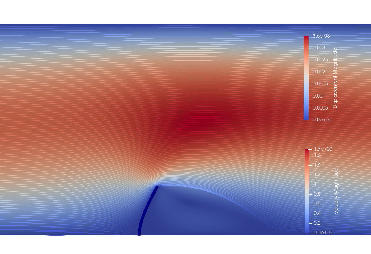

Note that the cantilever geometry is stored as the original undeformed geometry and a displacement field. In paraview, the geometry can be deformed to match the flow domain using the ‘Warp by Vector’ filter.
Relaxing the computation
In order to increase the speed of convergence, it is normally a good option to apply a relaxation
to the sub-iterations of the FSI problem. This is done by adding the following commands
BGS_RELAXATION= FIXED_PARAMETER
STAT_RELAX_PARAMETER= 0.8
to the FSI master config file. Running SU2 now would result in the following convergence history
+----------------------------------------------------------------+
|                        Multizone Summary                       |
+----------------------------------------------------------------+
|  Outer_Iter| avg[bgs][0]| avg[bgs][1]|MinVolume[0]|DeformIter[0|
+----------------------------------------------------------------+
|           0|   -0.298306|   -2.048554|  8.8212e-10|           0|
|           1|   -1.316281|   -2.740561|  8.4063e-10|          44|
|           2|   -2.215592|   -3.528252|  8.6618e-10|          44|
|           3|   -3.014938|   -4.639836|  8.7192e-10|          44|
|           4|   -3.732471|   -5.402349|  8.7309e-10|          44|
|           5|   -4.436227|   -5.790750|  8.7332e-10|          44|
|           6|   -5.137723|   -6.263485|  8.7337e-10|          44|
|           7|   -5.840368|   -6.711814|  8.7338e-10|          44|
|           8|   -6.536232|   -7.339662|  8.7338e-10|          44|
|           9|   -7.247336|   -7.555240|  8.7338e-10|          44|
|          10|   -7.946736|   -8.297281|  8.7338e-10|          44|
|          11|   -8.648240|   -8.586354|  8.7338e-10|          44|
|          12|   -9.353917|   -9.043231|  8.7338e-10|          44|
where the -9 convergence parameter is reached in almost half the iterations as per the non-relaxed case.
Printing the inner convergence
Sometimes, especially when things don’t work as expected, it’s interesting to visualize the convergence of each of the subproblems. This can be achieved enabling
WRT_ZONE_CONV = YES
in the main config file of the multizone problem, config_fsi_steady.cfg. In most cases we will not be interested on every single inner iteration of the fluid domain; we can use
SCREEN_WRT_FREQ_INNER = 10
in config_channel.cfg to limit the printout to every 10 iterations. The resulting screen output is the following:
+----------------------------------------------------------------+
|                     Zone 0 (Incomp. Fluid)                     |
+----------------------------------------------------------------+
|  Outer_Iter|  Inner_Iter|      rms[P]|      rms[U]|      rms[V]|
+----------------------------------------------------------------+
|           0|           0|   -4.799717|  -19.870540|  -32.000000|
|           0|          10|   -5.421646|   -4.859176|   -5.558343|
|           0|          20|   -6.200459|   -5.584293|   -6.120761|
|           0|          30|   -6.852188|   -6.205093|   -6.958953|
|           0|          40|   -7.502751|   -6.854100|   -8.034484|
|           0|          50|   -8.316190|   -7.662838|   -8.492639|
|           0|          60|   -9.153994|   -8.509430|   -9.696622|
|           0|          70|  -10.119472|   -9.498203|  -10.117162|
|           0|          80|  -11.035958|  -10.448171|  -11.143732|
|           0|          90|  -11.613994|  -10.982943|  -11.842820|
|           0|         100|  -12.264740|  -11.616077|  -12.556728|
|           0|         104|  -12.684964|  -12.046580|  -12.778620|
+-----------------------------------------------------------------------------+
|                              Zone 1 (Structure)                             |
+-----------------------------------------------------------------------------+
|  Outer_Iter|  Inner_Iter|      rms[U]|      rms[R]|      rms[E]|    VonMises|
+-----------------------------------------------------------------------------+
|           0|           0|   -1.121561|   -2.706864|   -4.419338|  2.2876e+03|
|           0|           1|   -1.708123|    1.269382|   -1.716845|  2.2429e+03|
|           0|           2|   -2.583705|    0.631041|   -3.175890|  2.2237e+03|
|           0|           3|   -2.508726|   -0.795411|   -5.686295|  2.0701e+03|
|           0|           4|   -2.751613|   -1.306797|   -6.550284|  2.0544e+03|
|           0|           5|   -3.147799|   -1.271416|   -6.914834|  2.0364e+03|
|           0|           6|   -2.962716|   -2.664273|   -7.800357|  2.0171e+03|
|           0|           7|   -4.083257|   -2.080066|   -8.553973|  2.0155e+03|
|           0|           8|   -4.522566|   -4.400710|  -11.005428|  2.0149e+03|
|           0|           9|   -7.252524|   -5.240218|  -14.876499|  2.0149e+03|
|           0|          10|  -10.834476|  -10.711888|  -23.634504|  2.0149e+03|
+----------------------------------------------------------------+
|                        Multizone Summary                       |
+----------------------------------------------------------------+
|  Outer_Iter| avg[bgs][0]| avg[bgs][1]|MinVolume[0]|DeformIter[0|
+----------------------------------------------------------------+
|           0|   -0.298306|   -2.048554|  8.8212e-10|           0|
...

+----------------------------------------------------------------+
|                     Zone 0 (Incomp. Fluid)                     |
+----------------------------------------------------------------+
|  Outer_Iter|  Inner_Iter|      rms[P]|      rms[U]|      rms[V]|
+----------------------------------------------------------------+
|          16|           0|  -15.808168|  -15.358431|  -15.769282|
|          16|          10|  -16.714759|  -16.074145|  -17.174991|
+-----------------------------------------------------------------------------+
|                              Zone 1 (Structure)                             |
+-----------------------------------------------------------------------------+
|  Outer_Iter|  Inner_Iter|      rms[U]|      rms[R]|      rms[E]|    VonMises|
+-----------------------------------------------------------------------------+
|          16|           0|  -11.937375|  -11.637725|  -25.999458|  1.8531e+03|
|          16|           1|  -15.794016|  -11.636749|  -28.541279|  1.8531e+03|
|          16|           2|  -16.165350|  -11.621837|  -28.528692|  1.8531e+03|
|          16|           3|  -16.056047|  -11.608302|  -28.544055|  1.8531e+03|
|          16|           4|  -16.156344|  -11.627675|  -28.565975|  1.8531e+03|
|          16|           5|  -16.204699|  -11.633976|  -28.581277|  1.8531e+03|
+----------------------------------------------------------------+
|                        Multizone Summary                       |
+----------------------------------------------------------------+
|  Outer_Iter| avg[bgs][0]| avg[bgs][1]|MinVolume[0]|DeformIter[0|
+----------------------------------------------------------------+
|          16|  -11.228939|   -9.130581|  8.7338e-10|          44|
where it can be observed that the multizone summary corresponds to the non-relaxed case presented first, and each of the subproblems are converged to a very high accuracy level.
References
\(^1\) Sanchez, R. (2018), A coupled adjoint method for optimal design in fluid-structure interaction problems with large displacements, PhD thesis, Imperial College London, DOI: 10.25560/58882
\(^2\) Matthies H. G. and Steindorf J. (2002), Partitioned but strongly coupled iteration schemes fornonlinear fluid–structure interaction, Computers & Structures, 80(27–30):199–1999.
Attribution
If you are using this content for your research, please kindly cite the following reference in your derived works:
Sanchez, R. et al. (2018), Coupled Adjoint-Based Sensitivities in Large-Displacement Fluid-Structure Interaction using Algorithmic Differentiation, Int J Numer Meth Engng, Vol 111, Issue 7, pp 1081-1107. DOI: 10.1002/nme.5700
-
This work is licensed under a Creative Commons Attribution 4.0 International License
