-
Inviscid Bump in a Channel
Inviscid Supersonic Wedge
Inviscid ONERA M6
Laminar Flat Plate
Laminar Cylinder
Turbulent Flat Plate
Transitional Flat Plate
Transitional Flat Plate for T3A and T3A-
Turbulent ONERA M6
Unsteady NACA0012
Epistemic Uncertainty Quantification of RANS predictions of NACA 0012 airfoil
Non-ideal compressible flow in a supersonic nozzle
Non-ideal compressible flows with physics-informed neural networks
Aachen turbine stage with Mixing-plane
-
Inviscid Hydrofoil
Laminar Flat Plate with Heat Transfer
Turbulent Flat Plate
Turbulent NACA 0012
Laminar Backward-facing Step
Laminar Buoyancy-driven Cavity
Streamwise Periodic Flow
Species Transport
Composition-Dependent model for Species Transport equations
Unsteady von Karman vortex shedding
Turbulent Bend with wall functions
Wind velocity and pollutant dispersion in a city
-
Static Fluid-Structure Interaction (FSI)
Dynamic Fluid-Structure Interaction (FSI) using the Python wrapper and a Nastran structural model
Static Conjugate Heat Transfer (CHT)
Unsteady Conjugate Heat Transfer
Solid-to-Solid Conjugate Heat Transfer with Contact Resistance
Incompressible, Laminar counterflow diffusion flame
Incompressible, Laminar Combustion Simulation
User Defined combustion model with Python
-
Unconstrained shape design of a transonic inviscid airfoil at a cte. AoA
Constrained shape design of a transonic turbulent airfoil at a cte. CL
Constrained shape design of a transonic inviscid wing at a cte. CL
Shape Design With Multiple Objectives and Penalty Functions
Unsteady Shape Optimization NACA0012
Unconstrained shape design of a two way mixing channel
Adjoint design optimization of a turbulent 3D pipe bend
Unsteady Shape Optimization NACA0012
| Written by | for Version | Revised by | Revision date | Revised version |
|---|---|---|---|---|
| @ScSteffen | 7.0.1 | @ScSteffen | 2020-01-27 | 7.0.1 |
Solver: |
|
Uses: |
|
Prerequisites: |
Unsteady NACA0012 |
Complexity: |
Basic |
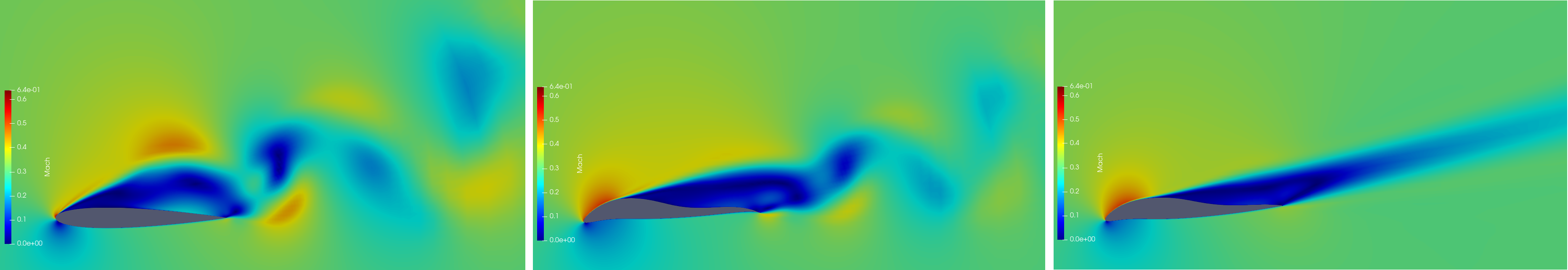 Figure (1): Baseline NACA0012 airfoil (left), optimized design using Square-windowing (middle) and optimized design using Hann-Square-windowing (right).
Goals
It is assumed, that the user is familiar with the shape optimization capabilities of SU2 in steady state flows, which are explained in the previous tutorials. Upon completing this tutorial, the user will be familiar with perfoming an optimization of a viscous, unsteady, periodic flow about a 2D geometry using the URANS equations. The specific geometry chosen for the tutorial is the classic NACA0012 airfoil. Consequently, the following capabilities of SU2 will be showcased in this tutorial.
- Windowed sensitivity calculation
- Unsteady adjoints
- Unsteady Optimization
This tutorial uses the windowing techniques explained in here, to compute meaningful optimization objectives. Hence it is recommended to read that tutorial first.
Resources
The resources for this tutorial can be found in the design/Unsteady_Shape_Opt_NACA0012 directory in the project website repository.
You will need the configuration file (unsteady_naca0012_opt.cfg) and the mesh file (unsteady_naca0012_FFD.su2).
The used mesh already contains an FFD-Box. For more information on how to set up an FFD-Box on your own, please follow this tutorial.
Tutorial
The following tutorial will walk you through the steps required when performing a shape optimization of the NACA0012 airfoil using SU2. The tutorial will also address procedures for parallel computations. To this end, it is assumed you have already obtained and compiled SU2_CFD and its adjoint capabilities. If you have yet to complete these requirements, please see the Download and Installation pages.
Background
This test case is for the NACA0012 airfoil in viscous unsteady flow. The NACA airfoils are two dimensional shapes for aircraft wings developed by the National Advisory Committee for Aeronautics (NACA, 1915-1958, predecessor of NASA). The NACA-4-Digit series is a set of 78 airfoil configurations which were created for wind-tunnel tests to explore the effect of different airfoil shapes on aerodynamic coefficients as drag or lift.
Mesh Description
The computational domain consists of a grid of 14495 quadrilaterals that surrounds the NACA0012 airfoil. Note that this is a very coarse mesh, and should one wish to obtain more accurate solutions for comparison with results in the literature, finer grids should be used.
Two boundary conditions are employed: The Navier-Stokes adiabatic wall condition on the wing surface and the far-field characteristic-based condition on the far-field marker.
Problem Setup
This problem will solve the flow about the airfoil with these conditions:
- Freestream Temperature = 293.0 K
- Freestream Mach number = 0.3
- Angle of attack (AOA) = 17.0 deg
- Reynolds number = 1E6
- Reynolds length = 1.0 m
- Number of time iterations: 2200
- Start of the windowed time-average: 1500
These subsonic flow conditions will cause a detached flow about the airfoil, that exhibts a vortex street and is therefore periodic for the baseline geometry. Depending on the windowing-function used to average the optimization objective, the flow about the optimized geometry will eventually be a steady state flow.
We want to solve an optimization problem with a time dependent system output, e.g. Drag. A meaningful objective and constraint function is therefore a time average over a period. The period average is approximated by a windowed time-average over a finite time-span \(M\)
\[\frac{1}{M}\int_0^M w(t/M)C_D(\sigma, t) \mathcal{d}t,\]where \(C_D(\sigma, t)\) denotes the drag coefficient. \(C_D(\sigma, t)\) depends on time \(t\) and the design parameters \(\sigma\). The window-function is denoted by \(w\). There are different windows available. Depending on their smoothness, they have different regularizing effects on the time-average and its sensitivity and therefore, the windowed time-average converges with different speed to the period-average. The following options are implemented:
| Window | Convergence Order | Convergence Order (sensitivity) |
|---|---|---|
SQUARE |
1 | 0 |
HANN |
3 | 2 |
HANN_SQUARE |
5 | 4 |
BUMP |
exponential | exponential |
For each optimization run, we have to compute the sensitivity of above windowed time-average, which reads
\[\frac{1}{M}\int_0^M w(t/M)\partial_\sigma C_D(\sigma, t) \mathcal{d}t.\]Figure 2 shows the time dependent drag and its sensitivity. As one can see, the amplitude of the drag sensitivity grows faster than linear. Roughly speaking, windowed time-average must converge faster than the amplitude of the oscillation grows to ensure convergence. This is the reason why Square-windowing is not a viable option for many application cases.
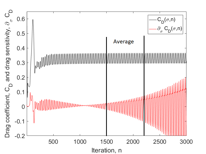 Figure (2): Instantaneous drag and drag sensitivity shown. The time frame to average the drag coefficient is in between iteration \(n_{tr} = 1500\) and \(N=2200\).
Using the midpoint rule for above integral, we arrive at the following constrained optimization problem
\[\min_{\sigma} \frac{1}{N-n_{tr}} \sum_{n_{tr}}^{N} w\left(\frac{n-n_{tr}}{N-n_{tr}}\right)C_D(\sigma,n)\] \[s.t. \qquad R(u^n) = 0 \qquad \forall n=1,\dots,N\] \[\qquad\qquad\frac{1}{N-n_{tr}} \sum_{n_{tr}}^{N} w\left(\frac{n-n_{tr}}{N-n_{tr}}\right)C_L(\sigma,n) \geq c\]The optimization constraint is given by the windowed time-averaged lift that should be greater than a specific value \(c\). We choose arbitrarily as \(c=0.96\), which is the windowed time-averaged lift of the baseline geometry. The time-span to average both lift and drag is given by \(M =N-n_{tr}\).
Configuration File Options
To compute the unsteady shape optimization, we set up the unsteady simulation according to our test case above. More information about setting up unsteady simulations can be found here
% -------- UNSTEADY SIMULATION -----------------%
%
TIME_DOMAIN = YES
%
% Numerical Method for Unsteady simulation
TIME_MARCHING= DUAL_TIME_STEPPING-2ND_ORDER
%
% Time Step for dual time stepping simulations (s)
TIME_STEP= 5e-4
%
% Maximum Number of physical time steps.
TIME_ITER= 2200
%
% Number of internal iterations (dual time method)
INNER_ITER= 400
%
% Time discretization for inner iteration.
TIME_DISCRE_FLOW= EULER_IMPLICIT
%
Furthermore, we specify the time frame to average the optimization objective. The starting iteration is given by WINDOW_START_ITER and the final iteration is the final time-step
of the simulation. The windowing-function can be specified using the option WINDOW_FUNCTION.
% Iteration to start the windowed time average
WINDOW_START_ITER = 1500
%
% Window-function to weight the time average. Options (SQUARE, HANN, HANN_SQUARE, BUMP), SQUARE is default.
WINDOW_FUNCTION = HANN_SQUARE
To compute the sensitivity of the optimization objective and constraint, SU2 uses an adjoint iterator. This means, sensitivies are calculated using a dual time-stepping method similar
to the one used for the direct simulation. Asymptotically, the convergence speed of the adjoint inner iteration matches the speed of the direct inner iteration. However,
it may happen that the adjoint inner iterator needs more iterations to reach a steady state. Make sure that the option INNER_ITER is chosen big enough in your test case to get
correct sensitivity results.
Note, that the adjoint iterator runs backwards in time, i.e. it starts at iteration given by UNST_ADJOINT_ITER and ends at iteration 0.
We set the start iteration to the final iteration of the direct run, i.e. UNST_ADJOINT_ITER = TIME_ITER = 2200.
The time to average the objective and constraint function is given by the option ITER_AVERAGE_OBJ. Here we set ITER_AVERAGE_OBJ=TIME_ITER-WINDOW_START_ITER=700.
%Iteration number to begin the reverse time integration in the direct solver for the unsteady adjoint.
UNST_ADJOINT_ITER = 2200
%
%Number of iterations to average the objective
ITER_AVERAGE_OBJ =  700
The optimization problem is given by the following known options.
% Optimization objective function with scaling factor
OPT_OBJECTIVE= DRAG * 1.0
%
% Optimization constraint functions with scaling factors, separated by semicolons
OPT_CONSTRAINT= ( LIFT > 0.96 ) * 1.0
%
% Box constraints for the design.
OPT_BOUND_UPPER= 0.05
OPT_BOUND_LOWER= -0.05
%
Running SU2
With each design iteration, the direct and adjoint solutions are used to compute the objective function and gradient, and the optimizer drives the shape changes with this information in order to minimize the objective. Each flow constraint requires the solution of an additional adjoint problem to compute its gradient (lift in this case). Two other SU2 tools are used in the design process here: SU2_DOT to compute the gradient from the adjoint surface sensitivities and input design space, and SU2_DEF to deform the computational mesh between design cycles. To run this case, follow these steps at a terminal command line:
-
Execute the shape optimization script by entering
$ shape_optimization.py -f unsteady_naca0012_opt.cfgat the command line, add
-n 4in case you want to run the optimization in parallel (4 cores). Again, note that Python, NumPy, and SciPy are all required to run the script. It is recommendend to run this optimization with at least 4 cores. However, if you don’t have a high number of cores available, you can reduce the time frame to optimize. One could choose for example% Maximum Number of physical time steps. TIME_ITER= 600 % % Iteration to start the windowed time average WINDOW_START_ITER = 350 % %Iteration number to begin the reverse time integration in the direct solver for the unsteady adjoint. UNST_ADJOINT_START_ITER = 600 % %Number of iterations to average the objective ITER_AVERAGE_OBJ = 250Note, that this configuration may produce different designs. To best showcase the difference between the windowing function, the original configuration is recommended.
-
The python script will drive the optimization process by executing flow solutions, adjoint solutions, gradient projection, geometry evaluations, and mesh deformation in order to drive the design toward an optimum. The optimization process will cease when certain tolerances set within the SciPy optimizer are met.
-
Solution files containing the flow and surface data will be written for each flow solution and adjoint solution and can be found in the DESIGNS directory that is created. The file named history_project.dat (or history_project.csv for ParaView) will contain the functional values of interest resulting from each evaluation during the optimization. The major iterations and function evaluations for the SLSQP optimizer will be written to the console during execution.
Results
One can see in Fig. (1) the baseline geometry alongside optimized designs created with different windowing functions.
The following figures display the shape optimization process with different windowing functions. The shape optimization performed with higher order windows, i.e. all windows exept the SQUARE-window perform well, whereas the
optimization computied using the SQUARE-window struggles to fulfill its optimization constraint.
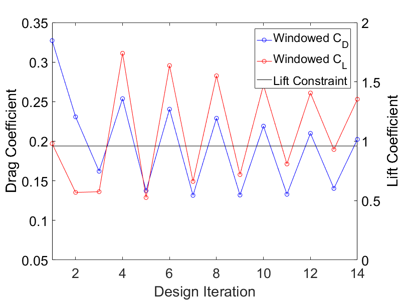 Figure (3): Shape optimization using Square-windowing.
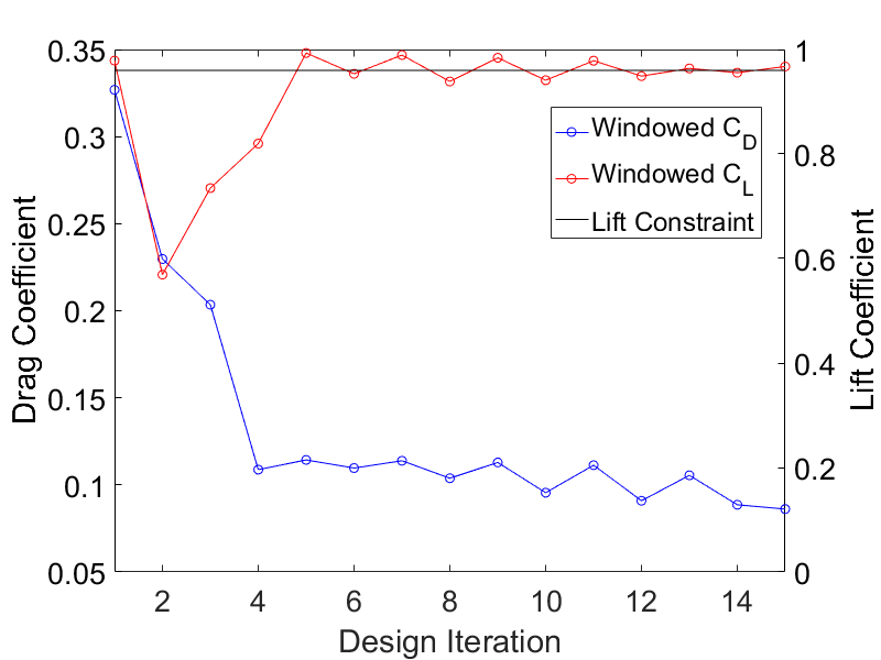 Figure (4): Shape optimization using Hann-windowing.
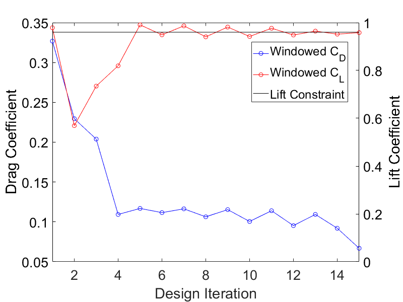 Figure (5): Shape optimization using Hann-Square-windowing.
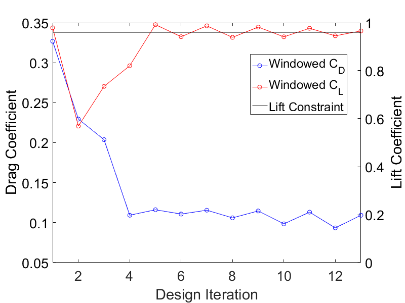 Figure (6): Shape optimization using Bump-windowing.