Streamwise Periodic Flow

Goals

Upon completing this tutorial, the user will be familiar with performing streamwise periodic simulations using the incompressible solver. All available features and limitations of streamwise periodic flow will be discussed. Consequently, the following capabilities of SU2 will be showcased in this tutorial:

• How to activate streamwise periodic flow without energy equation
• Switch between pressure drop and massflow prescription
• Adding the energy equation as true streamwise periodic flow and limitations
• Alternative to streamwise periodic temperature

Resources

The resources can be found in the incompressible_flow/Inc_Streamwise_Periodic directory in the tutorial repository. It contains the mesh file and two configuration files which will be discussed in this tutorial. Additionally, the script to create the used mesh with gmsh can be found that folder as well.

A more detailed theory description is available in the Docs here.

Tutorial

The following tutorial will walk you through the steps required when solving for a streamwise periodic flow using the incompressible solver. It is assumed you have already obtained and compiled the SU2_CFD code for a serial computation. If you have yet to complete these requirements, please see the Download and Installation pages. Users unfamiliar with using the incompressible solver can take a look at the other incompressible testcases, especially the Laminar Flat Plate with Heat Transfer.

Background

Flows through periodically repeating geometries can be approximated by just simulating a unit cell with streamwise periodicity. This model assumption of fully developed flow can be a justified approximation but has to be checked whether it is suitable. A 2D slice through a pin-fin heat-exchanger unit-cell is presented in this tutorial.

Problem Setup

This problem will solve for the incompressible RANS flow the following conditions:

• Density (constant) = 1045.0 kg/m^3
• Viscosity (constant) = 0.001385 kg/(m-s)
• Specific Heat Capacity (constant)= 3540.0 J/(kg-K)
• laminar Prandtl number (constant) = 11.7

As streamwise periodic flow is simulated, periodic boundaries are used instead of in-/outlets boundaries. The pin surfaces are heatlfux markers and are heated with 5e5 W/m^2. The remaining boundaries are symmetry markers.

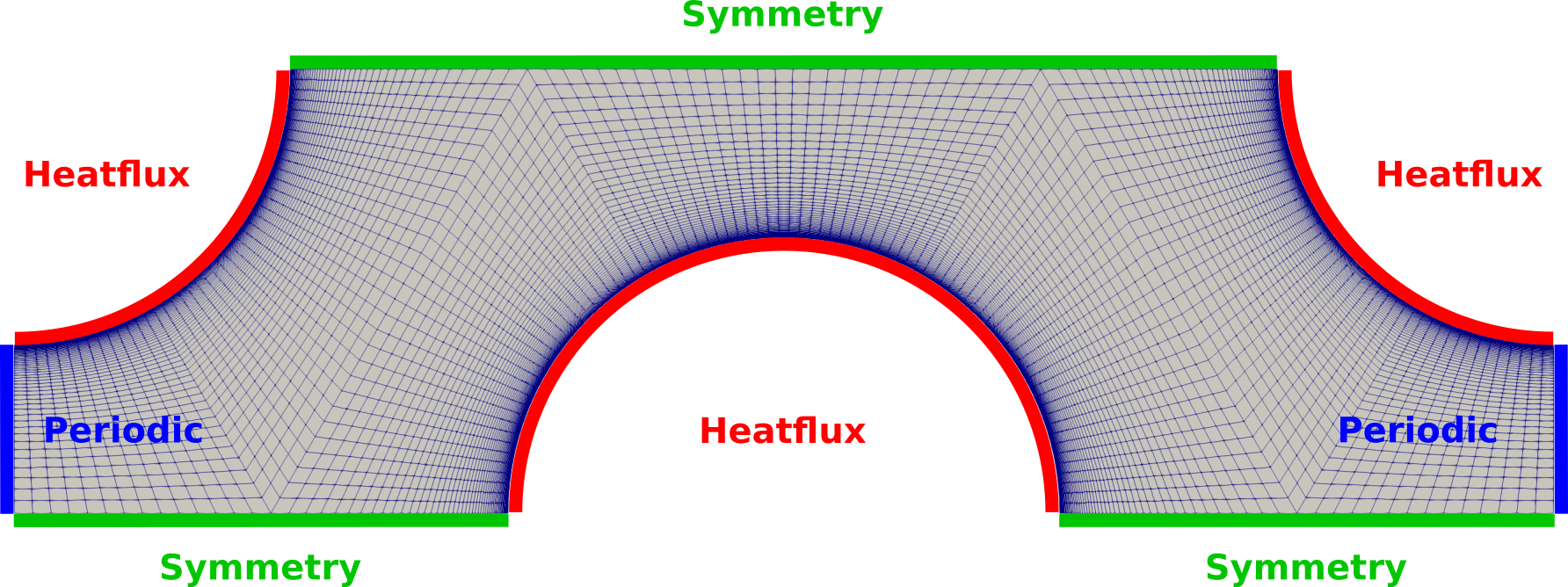
Figure (1): Figure of the computational mesh with the used boundary conditions.

Mesh Description

The computational mesh for the fluid has 8477 quad elements and is therefore fully structured. In- and outlet are meshed with 50 points and a progression such that y+<1 everywhere as the SST turbulence model is used. Each quarter-pin is meshed with 45 points in streamwise direction. A gmsh script is available to recreate/modify the mesh.

Configuration File Options

The available options for streamwise periodic flow are explained in this section.

Note that streamwise periodic flow is only available for the incompressible solver.

Using streamwise periodic flow requires having a periodic marker pair which can be set using MARKER_PERIODIC= (<inlet>, <outlet>, ...). The designated inlet has to be set first as a convention. The vector between periodic points on the in- and outlet has to be given as well in the case for translational periodicity as is discussed here. From the config_template.cfg:

% Periodic boundary marker(s) (NONE = no marker)
% Format: ( periodic marker, donor marker, rotation_center_x, rotation_center_y,
% rotation_center_z, rotation_angle_x-axis, rotation_angle_y-axis,
% rotation_angle_z-axis, translation_x, translation_y, translation_z, ... )
MARKER_PERIODIC= ( NONE )

For the rotation center and angle a zero has to provided such that in this case the marker definition looks like:

MARKER_PERIODIC= ( fluid_inlet, fluid_outlet, 0.0,0.0,0.0, 0.0,0.0,0.0, 0.0111544,0.0,0.0 )

At the moment, only one periodic marker pair is allowed, i.e. the combination with spanwise periodic flow is not possible.

KIND_STREAMWISE_PERIODIC activates streamwise periodic flow with the choice between a prescribed PRESSURE_DROP or MASSFLOW. With PRESSURE_DROP the prescribed value is set using STREAMWISE_PERIODIC_PRESSURE_DROP which also serves as a starting value if MASSFLOW is chosen.

Use STREAMWISE_PERIODIC_MASSFLOW for the respective massflow. With a precribed massflow the necessary pressure drop is determined iteratively, i.e. based on the difference between actual and target massflow an update to the pressure drop is estimated. This update can be relaxed using INC_OUTLET_DAMPING. Starting with a conservative guess to STREAMWISE_PERIODIC_PRESSURE_DROP and INC_VELOCITY_INIT will most likely a wise move.

If the energy equation is active then one can use STREAMWISE_PERIODIC_TEMPERATURE= YES if only heatflux and symmetry boundaries are used additional to the periodic markers. If that is not possible (i.e. if isothermal walls are used or a CHT interface is present), a heatsink at the outlet will automatically extract energy from the domain and will force the area-averaged inlet temperature to be identical to INC_TEMPERATURE_INIT. In order to support this process the user can provide an amount via STREAMWISE_PERIODIC_OUTLET_HEAT in Watts. If the value 0.0 (or none for that matter) is given, the integrated heat via MARKER_HEATFLUX is used.

Below the relevant excerpt from the config_template.cfg is shown.

% --------------------- STREAMWISE PERIODICITY DEFINITION ---------------------%
%
% Generally for streamwise periodicity one has to set MARKER_PERIODIC= (<inlet>, <outlet>, ...)
% appropriately as a boundary condition.
%
% Specify type of streamwise periodicity (default=NONE, PRESSURE_DROP, MASSFLOW)
KIND_STREAMWISE_PERIODIC= NONE
%
% Delta P [Pa] value that drives the flow as a source term in the momentum equations.
% Defaults to 1.0.
STREAMWISE_PERIODIC_PRESSURE_DROP= 1.0
%
% Target massflow [kg/s]. Necessary pressure drop is determined iteratively. 
% Initial value is given via STREAMWISE_PERIODIC_PRESSURE_DROP. Default value 1.0.
% Use INC_OUTLET_DAMPING as a relaxation factor. Default value 0.1 is a good start.
STREAMWISE_PERIODIC_MASSFLOW= 0.0
%
% Use streamwise periodic temperature (default=NO, YES)
% If NO, the heatflux is taken out at the outlet.
% This option is only necessary if INC_ENERGY_EQUATION=YES
STREAMWISE_PERIODIC_TEMPERATURE= NO
%
% Prescribe integrated heat [W] extracted at the periodic "outlet".
% Only active if STREAMWISE_PERIODIC_TEMPERATURE= NO.
% If set to zero, the heat is integrated automatically over all present MARKER_HEATFLUX.
% Upon convergence, the area averaged inlet temperature will be INC_TEMPERATURE_INIT.
% Defaults to 0.0.
STREAMWISE_PERIODIC_OUTLET_HEAT= 0.0
%

Additional SCREEN_OUTPUT for streamwise periodic flow is STREAMWISE_MASSFLOW, STREAMWISE_DP (i.e. Delta P or pressure drop) and STREAMWISE_HEAT which shows the heatflux integrated over HEATFLUX_MARKERS. By adding STREAMWISE_PERIODIC to HISTORY_OUTPUT those values are written the history file.

In this tutorial, 2 configuration files are provided which differ in the streamwise periodic options.

First, one of the simplest setups with a user provided pressure drop over the domain is chosen. Temperature periodicity is activated.

% --------------------- STREAMWISE PERIODICITY DEFINITION ---------------------%
%
KIND_STREAMWISE_PERIODIC= PRESSURE_DROP
STREAMWISE_PERIODIC_PRESSURE_DROP= 208.023676
%
STREAMWISE_PERIODIC_TEMPERATURE= YES
%

For the second configuration a massflow is prescribed. The initial pressure drop matches the final value but changes within the first iterations until the flow converges. Streamwise periodic temperature is deactivated so the outlet heatsink is used. In this case the 3 heatflux markers form a full circle which makes an exact computation of the introduced heatflux possible which can be then specified using the STREAMWISE_PERIODIC_OUTLET_HEAT. Note that an exact computation of this value is not always possible and also not necessary as the area-averaged inlet temperature must match INC_TEMPERATURE_INIT upon convergence which serves as an anchor for the temperature.

% --------------------- STREAMWISE PERIODICITY DEFINITION ---------------------%
%
KIND_STREAMWISE_PERIODIC= MASSFLOW
STREAMWISE_PERIODIC_MASSFLOW= 0.85
STREAMWISE_PERIODIC_PRESSURE_DROP= 208.023676
INC_OUTLET_DAMPING= 0.01
%
STREAMWISE_PERIODIC_TEMPERATURE= NO
% Computation of outlet heat: Heatflux * Area = Heatflux * pi * radius (as we have an accumulated full circle)
%                             5e5[W/m] * pi * 2e-3[m]
STREAMWISE_PERIODIC_OUTLET_HEAT= -3141.5926
%

Running SU2

To run this test case, follow these steps at a terminal command line:

1. Move to the directory containing the config files and the mesh files. Make sure that the SU2 tools were compiled, installed, and that their install location was added to your path.

2. Run the executable by entering

   $ SU2_CFD sp_pinArray_2d_dp_hf_tp.cfg
   

   at the command line for the first configuration. The filename makes use of some abbreviations: sp=streamwise periodic, 2d=2 dimensions, dp= delta p (prescribed), hf= heatflux (markers only), tp=temperature periodicity. The second configuration is run with

   $ SU2_CFD sp_pinArray_2d_mf_hf.cfg
   

   If SU2 is compiled with MPI support then you can execute SU2 in parallel

   $ mpirun -n <#cores> SU2_CFD sp_pinArray_2d_mf_hf.cfg
   

   where more than 8 cores do not provide major speedups due to the small mesh size.

3. SU2 will print residual updates with each outer iteration of the flow solver, and the simulation will terminate after reaching the specified convergence criteria.
4. Files containing the results will be written upon exiting SU2. The provided configuration files will write Paraview Multiblock files (.vtm) by default. The flow solution can be visualized in ParaView (.vtk) or Tecplot (.dat for ASCII) by setting the respective OUTPUT_FILES fields.

Results

The results for both simulations are discussed in this section. The difference is only visible for Temperature as both configurations end up having the same pressure drop and massflow by construction.

The visualizations are done using Paraview. To better visualize the differences, the Reflect (along symmetry axes) and Transform (at periodic interface) filters were used.

The velocity contour lines are shown in Figure (2). The turquoise line delimits the simulation domain. Demonstrating the computation of a fully developed flow on just a representative unit cell.

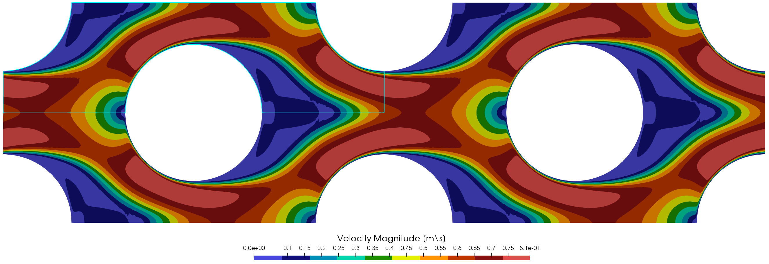
Figure (2): Velocity magnitude contour lines. The turquoise line delimits the simulation domain.

In Figure (3) the pressure is visualized. On the top the periodic pressure which is used as solution variable does not exhibit a pressure drop over the domain and can be interpreted to show only local phenomena. On the bottom the recovered (“physical”) pressure subtracts a linear term over the domain and therefore recovers the expected pressure drop. Note that negative pressures are possible in the incompressible solver as only pressure differences are used and the absolute pressure value is irrelevant.

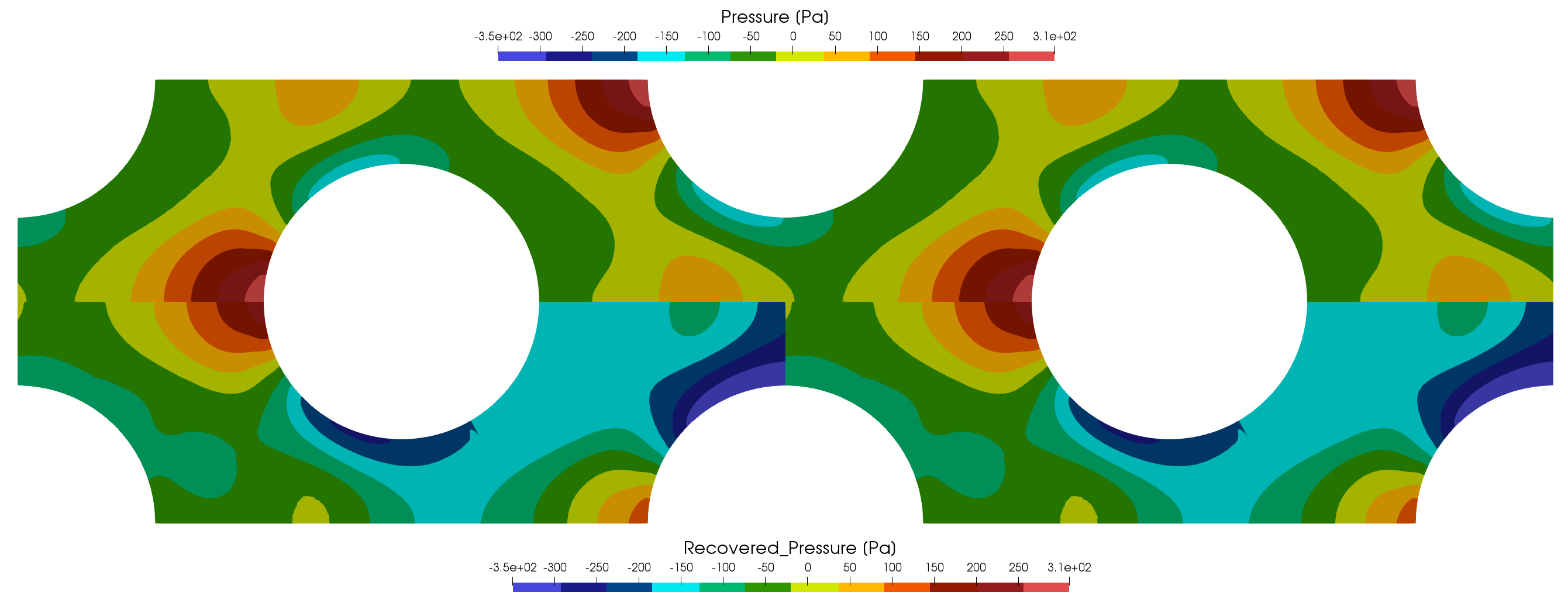
Figure (3): Pressure contour lines. Top: Periodic pressure that is used as solution variable. Bottom: Recovered pressure computed as postprocessing variable.

Similar to pressure is the handling of the streamwise periodic temperature. The visualization in Figure (4) is from the first discussed configuration. On the top the temperature filed is truly periodic and on the bottom the recoverd temperature allows a real world interpretation.

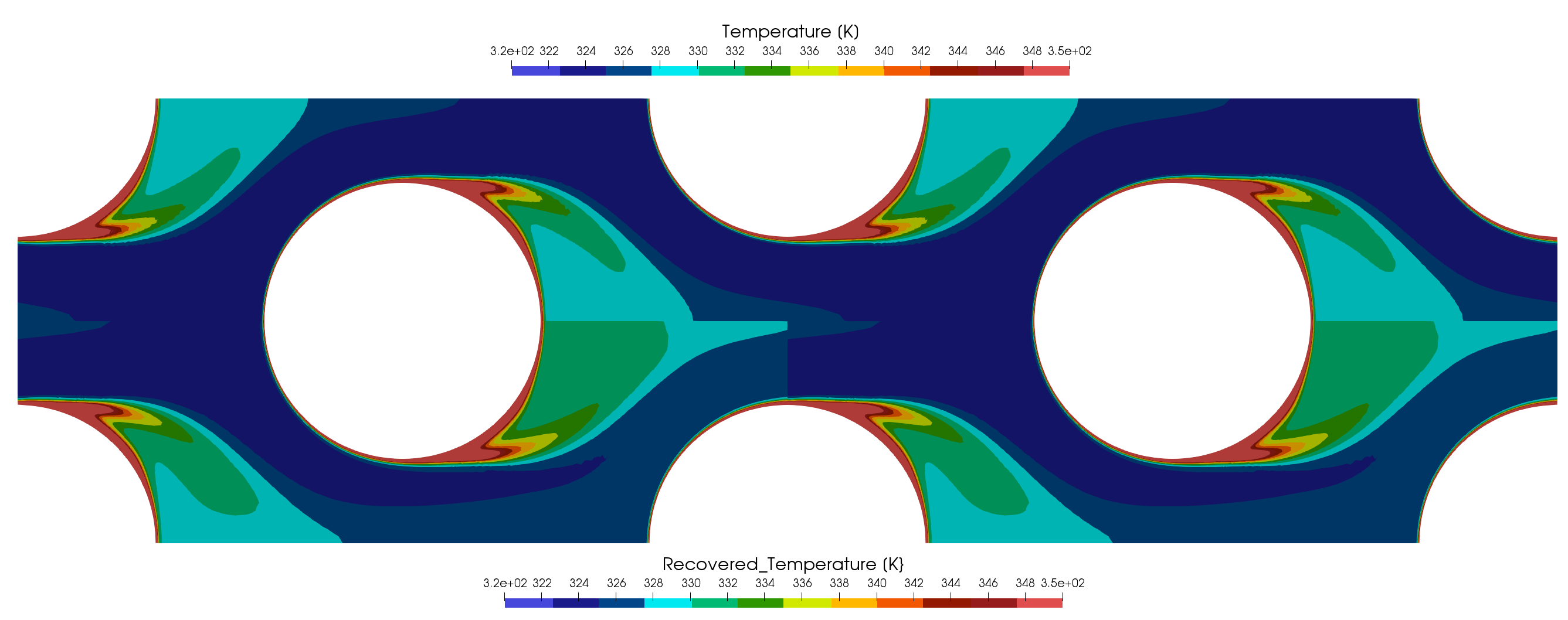
Figure (4): Temperature contour lines. Top: Periodic temperature that is used as solution variable. Bottom: Recovered temperature computed as postprocessing variable.

The temperature of the second configuration with the outlet heat sink is shown in Figure (5). Of course in this case only one temperature to be analyzed. Note that the temperature on the periodic in- and outlet are identical. The outlet heat sink is necessary to prevent an infinite rise in temperature in the case of only heatflux boundaries.

Figure (5): Temperature contour lines for simulation with an outlet heatsink.

Additional remarks

The extension to CHT cases is straight forward as the options in the fluid zone remain the same. STREAMWISE_PERIODIC_TEMPERATURE= NO has to be set as that feature is not compatible with the conjugate heat interfaces. A STREAMWISE_PERIODIC_OUTLET_HEAT can be provided by just integrating all heatflux markers of the combined fluid and heat zones. This of course does not handle possible isothermal walls but the excess energy is automatically balanced. A 2D CHT testcase based on the geometry presented here and a 3D CHT testcase are available in the testcases of SU2 under TestCases/incomp_navierstokes/streamwise_periodic/.

Temperature depended material properties are only reasonable to be used with STREAMWISE_PERIODIC_TEMPERATURE= NO as the solution variable Temperature would be truly periodic and therefore non-physical. The recovered Temperature would need to be used instead which is not available in the code at the moment.

The discrete adjoint does not work with KIND_STREAMWISE_PERIODIC= MASSFLOW in the moment. All other features are working with the discrete adjoint solver.