-
Inviscid Bump in a Channel
Inviscid Supersonic Wedge
Inviscid ONERA M6
Laminar Flat Plate
Laminar Cylinder
Turbulent Flat Plate
Transitional Flat Plate
Transitional Flat Plate for T3A and T3A-
Turbulent ONERA M6
Unsteady NACA0012
Epistemic Uncertainty Quantification of RANS predictions of NACA 0012 airfoil
Non-ideal compressible flow in a supersonic nozzle
Non-ideal compressible flows with physics-informed neural networks
Aachen turbine stage with Mixing-plane
-
Inviscid Hydrofoil
Laminar Flat Plate with Heat Transfer
Turbulent Flat Plate
Turbulent NACA 0012
Laminar Backward-facing Step
Laminar Buoyancy-driven Cavity
Streamwise Periodic Flow
Species Transport
Composition-Dependent model for Species Transport equations
Unsteady von Karman vortex shedding
Turbulent Bend with wall functions
Wind velocity and pollutant dispersion in a city
-
Static Fluid-Structure Interaction (FSI)
Dynamic Fluid-Structure Interaction (FSI) using the Python wrapper and a Nastran structural model
Static Conjugate Heat Transfer (CHT)
Unsteady Conjugate Heat Transfer
Solid-to-Solid Conjugate Heat Transfer with Contact Resistance
Incompressible, Laminar counterflow diffusion flame
Incompressible, Laminar Combustion Simulation
User Defined combustion model with Python
-
Unconstrained shape design of a transonic inviscid airfoil at a cte. AoA
Constrained shape design of a transonic turbulent airfoil at a cte. CL
Constrained shape design of a transonic inviscid wing at a cte. CL
Shape Design With Multiple Objectives and Penalty Functions
Unsteady Shape Optimization NACA0012
Unconstrained shape design of a two way mixing channel
Adjoint design optimization of a turbulent 3D pipe bend
Static Conjugate Heat Transfer (CHT)
| Written by | for Version | Revised by | Revision date | Revised version |
|---|---|---|---|---|
| @oleburghardt | 7.0.0 | @oleburghardt | 2021-01-18 | 7.0.8 |
Solver: |
|
Uses: |
|
User Guide: |
Basics of Multi-Zone Computations |
Prerequisites: |
Laminar Flat Plate with Heat Transfer |
Complexity: |
Advanced |
Goals
This tutorial builds on the laminar flat plate with heat transfer tutorial where incompressible solver with solution of the energy equation is introduced.
The following capabilities of SU2 will be showcased in this tutorial:
- Setting up a multiphysics simulation with Conjugate Heat Transfer (CHT) interfaces between zones
- Solution of the energy equation in solids
- Steady, 2D, laminar, incompressible, Navier-Stokes equations
- Discrete adjoint solutions and sensitivities for heat-related objective functions
The intent of this tutorial is to introduce a simple multiple physical zones case (one incompressible flow domain, three solid domains) where solvers are coupled by sharing a common interface.
Resources
The resources for this tutorial can be found in the multiphysics/steady_cht directory in the tutorial repository. You will need the configuration files for all physical zones (flow_cylinder.cfg, solid_cylinder1.cfg, solid_cylinder2.cfg, solid_cylinder3.cfg), the cofiguration file to invoke a multiphysics simulation run (cht_2d_3cylinders.cfg) and the mesh file (mesh_cht_3cyl_ffd.su2).
Tutorial
The following tutorial will walk you through the steps required when solving for a coupled CHT solution incorporating multiple physical zones. It is assumed you have already obtained and compiled the SU2_CFD code for a serial computation. If you have yet to complete these requirements, please see the Download and Installation pages.
Background
CHT simulations become important when we cannot assume an isomthermal wall boundary or when we even have no suitable temperature distribution estimate at hand. This is typically the case when a wall happens to be the boundary of a solid (e.g. metal) part and heat transfer across the boundary cannot be neglected.
The correct interface temperature distribution has then to be found by the simulation run as well, that is, by coupling energy quantities in all zones.
Problem Setup
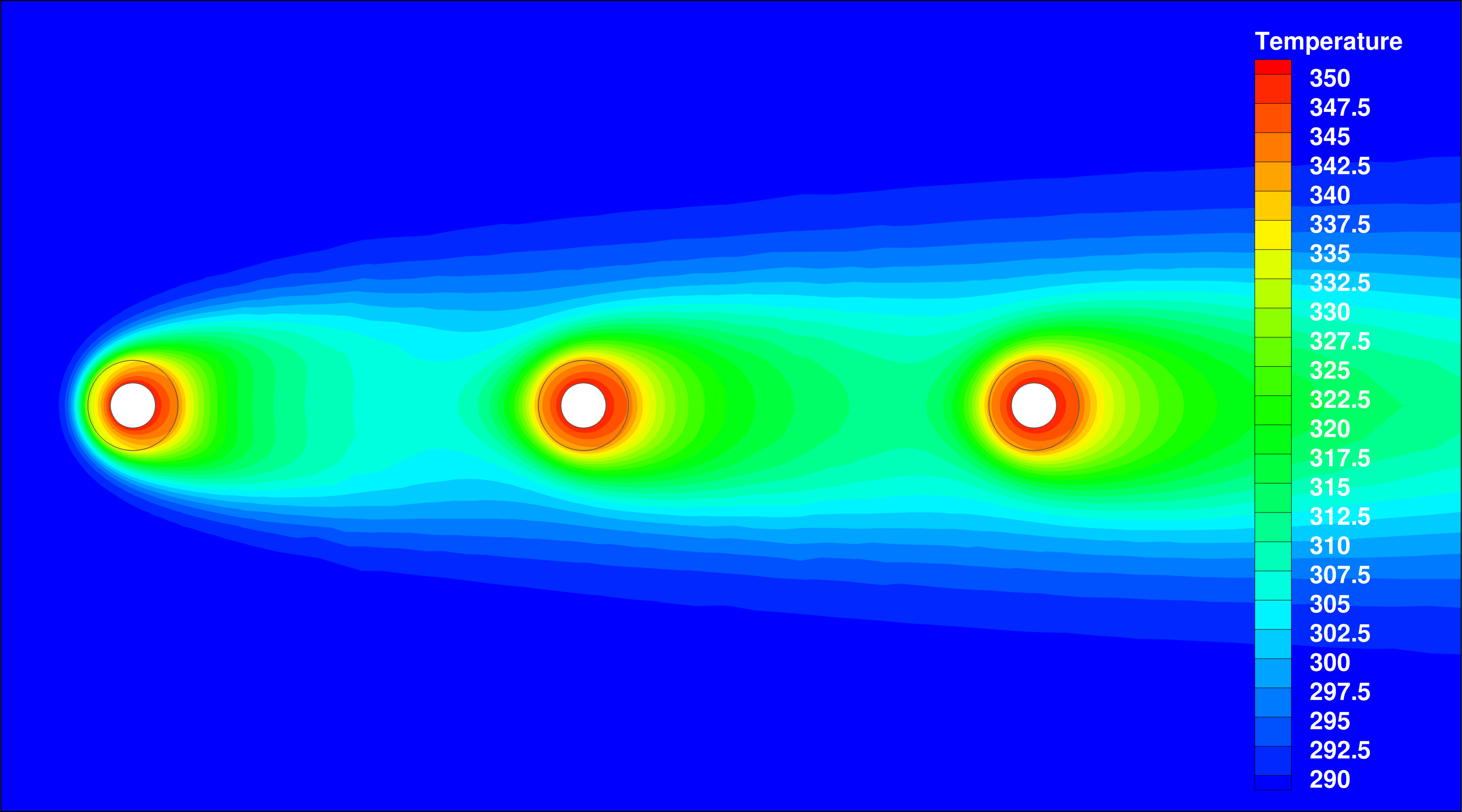
This problem will solve for the incompressible flow over three cylinders as well as for the heat equation in all cylinders that are coupled by energy conservation across the interfaces.
The following flow conditions that are set to match the Reynolds number of 40. For hollow cylinders with outer diameters of 1m:
- Density (variable) = 0.000210322 kg/m^3
- Farfield Velocity Magnitude = 3.40297 m/s
- Farfield Flow Direction, unit vector (x,y,z) = (1.0, 0.0, 0.0)
- Farfield Temperature = 288.15 K
- Viscosity (constant) = 1.7893e-05 kg/(m-s)
- Specific heat (constant) = 1004.703 J/(kg-K)
- Prandtl Number (constant) = 0.72
The hollow cylinders will have the same material properties for its density (set to 0.00042 kg/m^3) and specific heat but a 4 times higher thermal conductivity of 0.1 W/(m-K).
A constant temperature boundary condition of 350 K on the inner core drives the heating in the solid and fluid zones.
Mesh Description
The computational mesh for the fluid zone is composed 33700 elements (quad-dominant). The far-field boundary contains 80 line elements and the cylinders surfaces all have 400 line elemtents.
The meshes for all three cylinders are composed of 4534 elements (quad-dominant) each, their inner diamaters are composed of 40 line elements, at their outer diamaters the mesh matches the one of the fluid zone.
 Figure (1): Figure of the computational mesh with all four physical zones.
Uniform velocity boundary conditions are used for the farfield.
Configuration File Options
Several of the key configuration file options for this simulation are highlighted here. First we show how we start a multiphysics simulation run incorporating CHT by choosing the following options in a main config file cht_2d_3cylinders.cfg (see https://su2code.github.io/docs_v7/Multizone how to setup a multiphysics simulation in general):
MARKER_ZONE_INTERFACE= (cylinder_outer1, cylinder_inner1, cylinder_outer2, cylinder_inner2, cylinder_outer3, cylinder_inner3)
%
%
MARKER_CHT_INTERFACE= (cylinder_outer1, cylinder_inner1, cylinder_outer2, cylinder_inner2, cylinder_outer3, cylinder_inner3)
By setting MARKER_CHT_INTERFACE for the outer diameters, temperature and heat flux data will be exchanged between the solvers at these boundaries in each outer iteration.
As in the laminar flat plate with heat transfer tutorial, we activate the energy equation in the flow domain config (flow_cylinder.cfg) but this time we allow for variable density as the heat input causes a non-neglectable influence on the density:
% ---------------- INCOMPRESSIBLE FLOW CONDITION DEFINITION -------------------%
%
% Density model within the incompressible flow solver.
% Options are CONSTANT (default), BOUSSINESQ, or VARIABLE. If VARIABLE,
% an appropriate fluid model must be selected.
INC_DENSITY_MODEL= VARIABLE
%
% Solve the energy equation in the incompressible flow solver
INC_ENERGY_EQUATION = YES
With the energy equation with variable density active, a value for the specific heat at constant pressure (Cp) should be specified as well as an appropriate fluid model that relates temperature and density.
% ---- IDEAL GAS, POLYTROPIC, VAN DER WAALS AND PENG ROBINSON CONSTANTS -------%
%
% Fluid model (STANDARD_AIR, IDEAL_GAS, VW_GAS, PR_GAS,
%              CONSTANT_DENSITY, INC_IDEAL_GAS)
FLUID_MODEL= INC_IDEAL_GAS
%
% Specific heat at constant pressure, Cp (1004.703 J/kg*K (air)).
% Incompressible fluids with energy eqn. only (CONSTANT_DENSITY, INC_IDEAL_GAS).
SPECIFIC_HEAT_CP= 1004.703
The config files for the solid zones are quite short and mostly identical. E.g. for the first cylinder in upstream direction (solid_cylinder1.cfg), we have to invoke the heat equation solver by
% Physical governing equations (EULER, NAVIER_STOKES,
%                               WAVE_EQUATION, HEAT_EQUATION, FEM_ELASTICITY,
%                               POISSON_EQUATION)
SOLVER= HEAT_EQUATION
and then set in inner (core) diameter temperature to 350 K (as mentioned above), that is we set
% -------------------- BOUNDARY CONDITION DEFINITION --------------------------%
%
MARKER_ISOTHERMAL= ( core1, 350.0 )
The solid’s material properties are chosen as follows.
% Solid density (kg/m^3)
MATERIAL_DENSITY= 0.00021
%
% Solid specific heat (J/kg*K)
SPECIFIC_HEAT_CP = 1004.703
%
% Solid thermal conductivity (W/m*K)
KT_CONSTANT= 0.1028
Running SU2
The CHT simulation for the provided mesh will execute relatively quick, given that the coupled outer loop has to converge to a interface temperature solution as well. To run this test case, follow these steps at a terminal command line:
- Move to the directory containing the config files and the mesh files. Make sure that the SU2 tools were compiled, installed, and that their install location was added to your path.
-
Run the executable by entering
$ SU2_CFD cht_2d_3cylinders.cfgat the command line.
- SU2 will print residual updates with each outer iteration of the flow solver, and the simulation will terminate after reaching the specified convergence criteria.
- Files containing the results will be written upon exiting SU2. The flow solution can be visualized in ParaView (.vtk) or Tecplot (.dat for ASCII).
Discrete adjoint solutions
For optimization purposes, SU2 can perform discrete adjoint solutions for multiphysics simulations as well. Given the solution files from all the zones, we only have to change MATH_PROBLEM from DIRECT to
% Mathematical problem (DIRECT, CONTINUOUS_ADJOINT, DISCRETE_ADJOINT)
MATH_PROBLEM= DISCRETE_ADJOINT
in the main config file.
SU2 will then compute coupled discrete adjoint solutions for all physical zones for a given objective function. Note that all cross dependencies from the CHT coupling at the interfaces are captured by default to give accurate sensitivities later on.
As for this test case, the objective function will be the sum of all integrated heat fluxes at the CHT interfaces. This can be done by setting
% For a weighted sum of objectives: separate by commas, add OBJECTIVE_WEIGHT and MARKER_MONITORING in matching order.
OBJECTIVE_FUNCTION= TOTAL_HEATFLUX
% Marker(s) of the surface where the functional (Cd, Cl, etc.) will be evaluated
MARKER_MONITORING= (cylinder_outer1, cylinder_outer2, cylinder_outer3)
in flow_cylinder.cfg and
% Marker(s) of the surface where the functional (Cd, Cl, etc.) will be evaluated
MARKER_MONITORING= ( NONE )
in solid_cylinder1.cfg, solid_cylinder2.cfg and solid_cylinder3.cfg.
One could also set objective functions in all the solid config files seperately which would in the end give same results.
Based on all four solution files from the different zones (solution_flow_0.dat and so on), we start the discrete adjoint run by entering
$ SU2_CFD_AD cht_2d_3cylinders.cfg
Results and Validation
Surface node sensitivities can be obtained from the discrete adjoint solutions via
$ cp restart_adj_totheat_0.dat solution_adj_totheat_0.dat
$ cp restart_adj_totheat_1.dat solution_adj_totheat_1.dat
$ cp restart_adj_totheat_2.dat solution_adj_totheat_2.dat
$ cp restart_adj_totheat_3.dat solution_adj_totheat_3.dat
$ SU2_DOT_AD cht_2d_3cylinders.cfg
which are written to surface output files for each zone. Sensitivites from surface_sens_0.dat are shown as blue arrows, for all solid zones (surface_sens_1.dat, surface_sens_2.dat, surface_sens_3.dat) as red arrows.
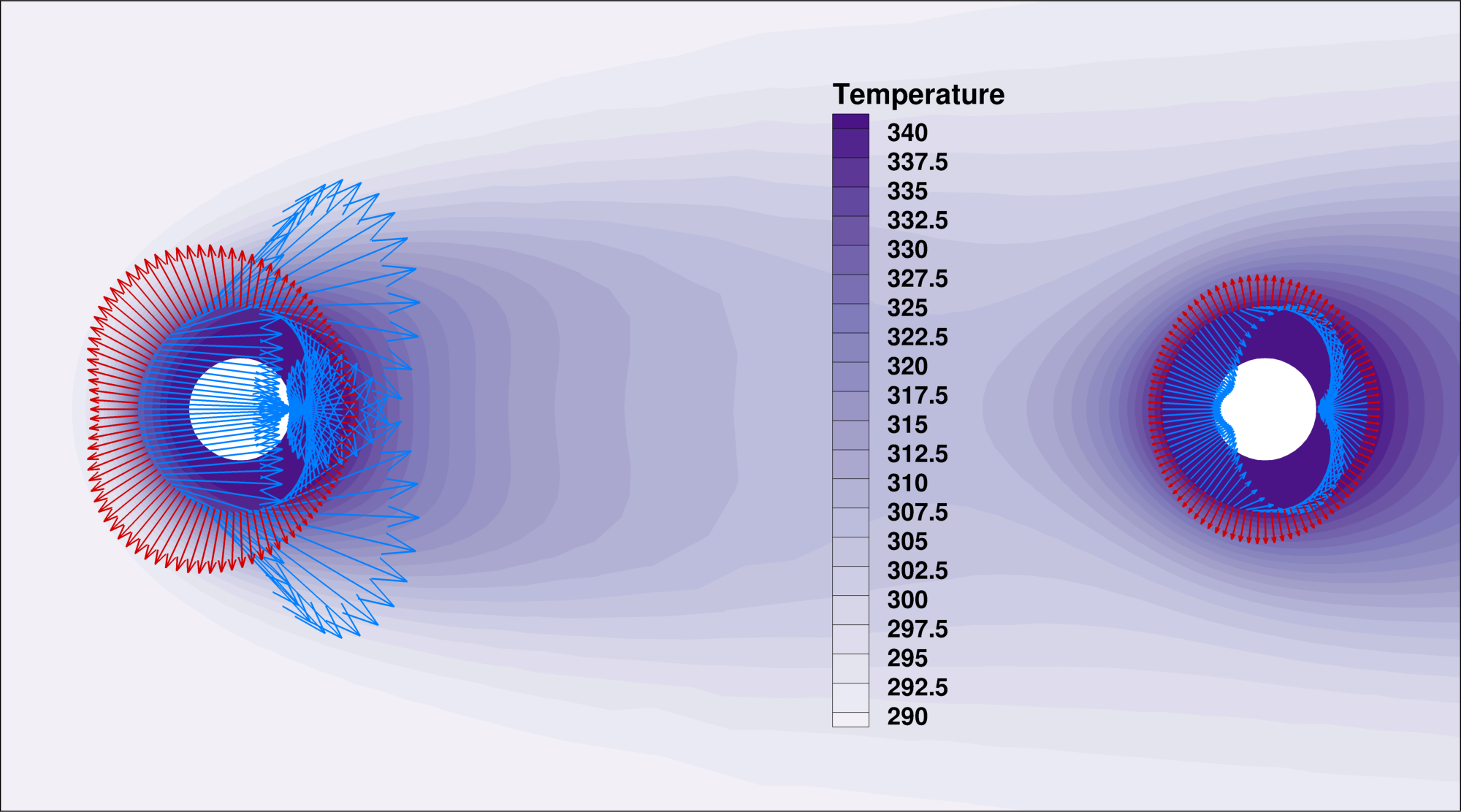 Figure (2): Heat flux sensitivities obtained from the discrete adjoint flow solution (blue) and the discrete adjoint heat solutions (red), their sum giving the correct result. Note the sensitivity change in downstream direction in both directions and magnitude.
In order to validate the sensitivities (and therefore the discrete adjoint solutions, too), a free-form deformation box was already created around the first heated cylinder, to project all sensitivities onto one design variable (a FFD box control point) to check the obtained derivative against finite differences.
 Figure (3): FFD box of degree 24x1.
The upper middle control point at (12,1), moving into y-direction, is then used to define a single design parameter modifying the shape. This can be done by
DV_KIND= FFD_CONTROL_POINT_2D
DV_MARKER= ( cylinder_outer1, cylinder_inner1 )
DV_PARAM= ( MAIN_BOX, 12, 1, 0.0, 1.0 )
as in the main config file. The derivative of the integrated heat flux with respect to this design veriable was thus alsp automatically computed and written to of_grad_0.dat and of_grad_1.dat; the other to cylinders are giving no direct contribution as their shape is not affected).
We will check the derivative (0.152507 + 0.234148 + 0.0 + 0.0 = 0,386655) against finite differences at magnitudes from 1.0e-2 to 1.0e-6. To this end, we have to deform the multizone mesh by setting
DV_VALUE= 0.00001
and running
$ SU2_DEF cht_2d_3cylinders.cfg
which will produce the deformed multizone mesh mesh_cht_3cyl_out.su2, on which the integrated heatflux can be recomputed (analogously for other magnitudes). Relative errors to the value generated from discrete adjoints are given below.
| magnitude | heatflux value | FD derivative | rel. error (%) |
|---|---|---|---|
| 1.0e-2 | -31.89331058028049 | 0,390077422 | 0,8861153 |
| 1.0e-3 | -31.89682435269217 | 0.387001813 | 0.0906675 |
| 1.0e-4 | -31.89717268560501 | 0.386688997 | 0.0097636 |
| 1.0e-5 | -31.89720748792119 | 0.38665835 | 0.0018381 |
| 1.0e-6 | -31.89721096784924 | 0.38665548 | 0.001095 |