Inviscid ONERA M6

Goals

Upon completing this tutorial, the user will be familiar with performing a simulation of external, inviscid flow around a 3D geometry. The specific geometry chosen for the tutorial is the classic ONERA M6 wing. Consequently, the following capabilities of SU2 will be showcased in this tutorial:

• Steady, 3D Euler equations
• Multigrid
• JST convective scheme in space (2nd-order, centered)
• Euler implicit time integration
• Euler Wall, Symmetry, and Far-field boundary conditions
• Code parallelism (recommended)

We will also discuss the details for setting up 3D flow conditions and some of the multigrid options within the configuration file.

Resources

The resources for this tutorial can be found in the compressible_flow/Inviscid_ONERAM6 directory in the tutorial repository. You will need the configuration file (inv_ONERAM6.cfg) and the mesh file (mesh_ONERAM6_inv_ffd.su2).

Tutorial

The following tutorial will walk you through the steps required when solving for external flow past the ONERA M6 using SU2. The tutorial will also address procedures for both serial and parallel computations. It is assumed that you have already obtained and compiled the SU2_CFD code for a serial computation or both the SU2_CFD and SU2_SOL codes for a parallel computation. If you have yet to complete these requirements, please see the Download and Installation pages.

Background

This test case is for the ONERA M6 wing in inviscid flow. The ONERA M6 wing was designed in 1972 by the ONERA Aerodynamics Department as an experimental geometry for studying three-dimensional, high Reynolds number flows with some complex flow phenomena (transonic shocks, shock-boundary layer interaction, separated flow). It has become a classic validation case for CFD codes due to the relatively simple geometry, complicated flow physics, and availability of experimental data. This test case will be performed in inviscid flow at a transonic Mach number.

Problem Setup

This problem will solve the for the flow past the wing with these conditions:

• Freestream Pressure = 101325.0 N/m2
• Freestream Temperature = 288.15 K
• Freestream Mach number = 0.8395
• Angle of attack (AOA) = 3.06 deg

These transonic flow conditions will cause the typical “lambda” shock along the upper surface of the lifting wing.

Mesh Description

The computational domain is a large parallelepiped with the wing half-span mounted on one boundary in the x-z plane. The mesh consists of 582,752 tetrahedral elements and 108,396 nodes. Three boundary conditions are employed: Euler wall on the wing surface, a far-field characteristic-based condition on the far-field markers, and a symmetry boundary condition for the marker where the wing half-span is attached. The symmetry condition acts to mirror the flow about the x-z plane, reducing the complexity of the mesh and the computational cost. Images of the entire domain and the triangular elements on the wing surface are shown below.

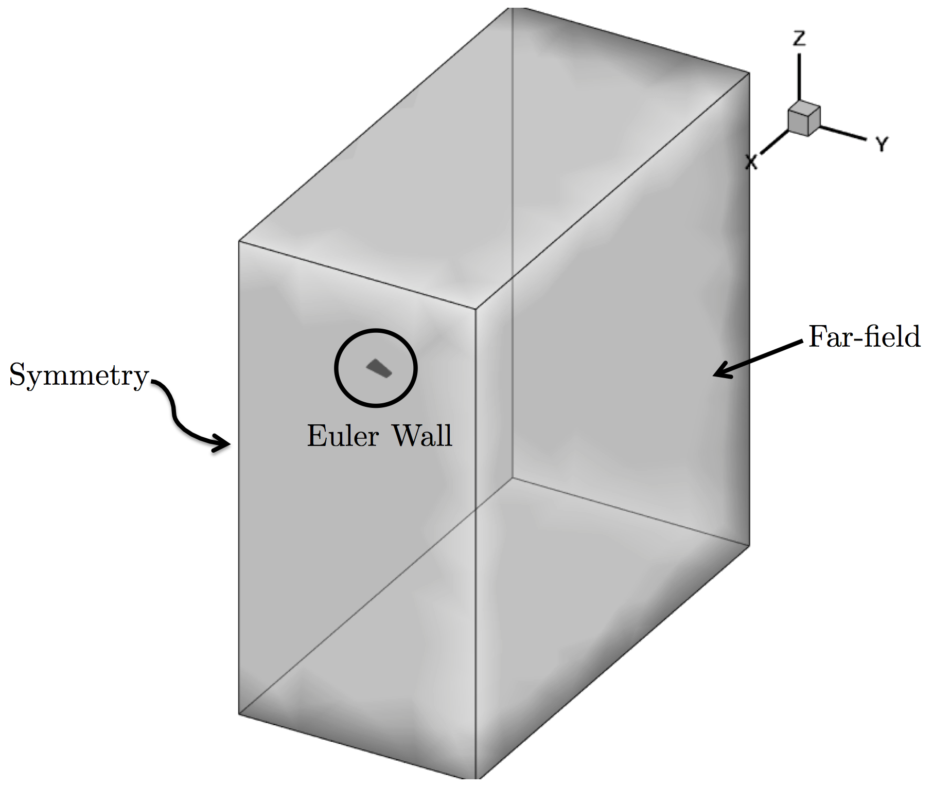Figure (1): Far-field view of the computational mesh with boundary conditions.

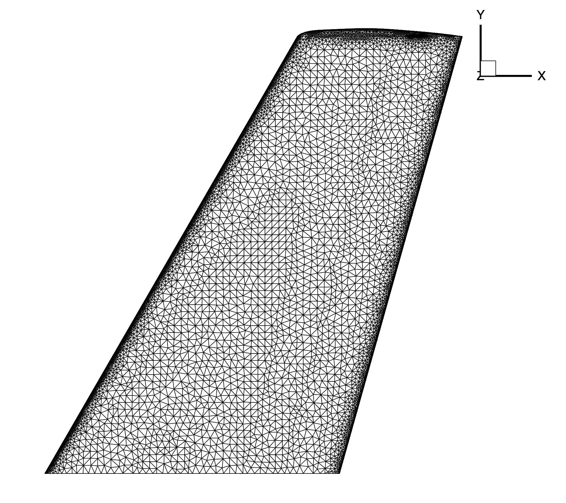Figure (2): Close-up view of the unstructured mesh on the top surface of the ONERA M6 wing.

Configuration File Options

Several of the key configuration file options for this simulation are highlighted here. The following describes how to set up 3D flow conditions for compressible flow in SU2:

% -------------------- COMPRESSIBLE FREE-STREAM DEFINITION --------------------%
%
% Mach number (non-dimensional, based on the free-stream values)
MACH_NUMBER= 0.8395
%
% Angle of attack (degrees)
AOA= 3.06
%
% Side-slip angle (degrees)
SIDESLIP_ANGLE= 0.0
%
% Free-stream pressure (101325.0 N/m^2 by default)
FREESTREAM_PRESSURE= 101325.0
%
% Free-stream temperature (288.15 K by default)
FREESTREAM_TEMPERATURE= 288.15

For an inviscid problem such as this, the flow conditions are completely defined by an input Mach number, flow direction, freestream pressure, and freestream temperature. The input Mach number is transonic at 0.8395. The freestream temperature and pressure have been set to standard sea level values for air at 101325.0 N/m^2 and 288.15 K, respectively. The flow field will be initialized to these freestream values everywhere in the domain.

Lastly, it is very important to note the definition of the freestream flow direction in 3D. The default freestream direction (AOA = 0.0 degrees and SIDESLIP_ANGLE = 0.0 degrees) is aligned with the positive x-axis without any components in the y- or z-directions. Referring to Figure (1), we see that AOA = 3.06 degrees will result in a non-zero freestream velocity in the positive z-direction. While zero for this problem, setting the SIDESLIP_ANGLE to a non-zero value would result in a non-zero velocity component in the y-direction. In 2D, the flow is in the x-y plane. While the default freestream direction is still along the positive x-axis, a non-zero AOA value for 2D problems will result in a non-zero freestream velocity in the y-direction. The SIDESLIP_ANGLE variable is unused in 2D.

The user can define reference values for non-dimensionalization and force computation purposes:

% ---------------------- REFERENCE VALUE DEFINITION ---------------------------%
%
% Reference origin for moment computation
REF_ORIGIN_MOMENT_X = 0.25
REF_ORIGIN_MOMENT_Y = 0.00
REF_ORIGIN_MOMENT_Z = 0.00
%
% Reference length for pitching, rolling, and yaMAIN_BOX non-dimensional moment
REF_LENGTH= 1.0
%
% Reference area for force coefficients (0 implies automatic calculation)
REF_AREA= 0
%
% Flow non-dimensionalization (DIMENSIONAL, FREESTREAM_PRESS_EQ_ONE,
%                              FREESTREAM_VEL_EQ_MACH, FREESTREAM_VEL_EQ_ONE)
REF_DIMENSIONALIZATION= FREESTREAM_VEL_EQ_ONE

SU2 accepts arbitrary reference values for computing the force coefficients. A reference area can be supplied by the user for the calculation of force coefficients (e.g., a trapezoidal wing area) with the REF_AREA variable. If REF_AREA is set equal to zero, as for the ONERA M6, a reference area will be automatically calculated by summing all surface normal components in the positive z-direction on the monitored markers for 3D calculations.

For this ONERA M6 case, SU2 performs a non-dimensional simulation (REF_DIMENSIONALIZATION= FREESTREAM_VEL_EQ_ONE). This option controls your non-dim. scheme for compressible flow problems. If you wish to perform a dimensional simulation you can pick the DIMENSIONAL option. For non-dimensionalization case FREESTREAM_PRESS_EQ_ONE the free-stream values at the far-field will be (pressure = 1.0, density = 1.0, temperature = 1.0). For FREESTREAM_VEL_EQ_MACH the free-stream values at the far-field will be (velocity = Mach number, density = 1.0, temperature = 1.0) and for FREESTREAM_VEL_EQ_ONE the free-stream values at the far-field will be (velocity = 1.0, density = 1.0, temperature = 1.0).

Finally, we discuss some important multigrid options:

% -------------------------- MULTIGRID PARAMETERS -----------------------------%
%
% Multi-Grid Levels (0 = no multi-grid)
MGLEVEL= 3
%
% Multi-grid cycle (V_CYCLE, W_CYCLE, FULLMG_CYCLE)
MGCYCLE= W_CYCLE
%
% Multi-Grid PreSmoothing Level
MG_PRE_SMOOTH= ( 1, 2, 3, 3 )
%
% Multi-Grid PostSmoothing Level
MG_POST_SMOOTH= ( 0, 0, 0, 0 )
%
% Jacobi implicit smoothing of the correction
MG_CORRECTION_SMOOTH= ( 0, 0, 0, 0 )
%
% Damping factor for the residual restriction
MG_DAMP_RESTRICTION= 0.9
%
% Damping factor for the correction prolongation
MG_DAMP_PROLONGATION= 0.9

SU2 contains an agglomeration multigrid algorithm for convergence acceleration (a Full-Approximation Storage, or FAS, multigrid) where the original mesh is automatically agglomerated into a series of coarser representations, and smoothing iterations are performed on all mesh levels with each non-linear solver iteration in order to provide a better residual update. The user can set the number of multigrid levels using the MGLEVEL option. If this is set to zero, multigrid will be turned off, and only the original (fine) mesh will be used. An integer number of levels can be chosen. The ONERA M6 test case uses 3 levels of coarser meshes along with the original mesh for a total of 4 mesh levels. The type of cycle (V or W) can also be specified, and in general, while more computationally intensive, a W-cycle provides better convergence rates. There are additional tuning parameters that control the number of pre- and post-smoothing iterations on each level (MG_PRE_SMOOTH, MG_POST_SMOOTH, and MG_CORRECTION_SMOOTH), along with damping factors that can help in achieving stability (MG_DAMP_RESTRICTION and MG_DAMP_PROLONGATION).

It is important to note that the performance of the multigrid algorithm is highly-dependent on the initial grid and that the agglomeration is impacted by parallel partitioning: considerable tuning and experimentation with these parameters can be required. If you are having trouble tuning the multigrid, it is recommended to turn it off (set MGLEVEL = 0) and to try with a higher CFL number on the fine grid alone while converging the implicit system to a tighter tolerance (use the LINEAR_SOLVER_ERROR and LINEAR_SOLVER_ITER options).

In addition to aggressive multigrid settings for this case, we also apply automatic CFL adaption, which allows for ramping of the CFL number to very high values. This results in rapid convergence of the problem after approximately 100 iterations. The CFL adaption is enabled using the following options:

%
% Adaptive CFL number (NO, YES)
CFL_ADAPT= YES
%
% Parameters of the adaptive CFL number (factor down, factor up, CFL min value,
%                                        CFL max value )
CFL_ADAPT_PARAM= ( 0.1, 2.0, 100.0, 1e10 )

First, we set CFL_ADAPT= YES to activate CFL adaption. The parameters for the adaption are set with CFL_ADAPT_PARAM in order to control the multiplicative factors to increase or decrease the CFL with each iteration (depending on the success of each nonlinear iteration) as well as minimum and maximum bounds on the allowable CFL. For Euler and laminar Navier-Stokes problems, an aggressive strategy that doubles the CFL up to a high max (here 1e10) is typically possible. For RANS cases, more conservative values are suggested (increase factor of 1.2 and a max of 1e3).

Running SU2

Instructions for running this test case are given here for both serial and parallel computations. The computational mesh is rather large, so if possible, performing this case in parallel is recommended.

In Serial

The wing simulation is relatively large for a single-core calculation, but is still reasonable due to the high convergence rate of this inviscid case. To run this test case, follow these steps at a terminal command line:

1. Move to the directory containing the config file (inv_ONERAM6.cfg) and the mesh file (mesh_ONERAM6_inv_ffd.su2). Make sure that the SU2 tools were compiled, installed, and that their install location was added to your path.

2. Run the executable by entering

    $ SU2_CFD inv_ONERAM6.cfg
   

   at the command line.

3. SU2 will print residual updates with each iteration of the flow solver, and the simulation will terminate after reaching the specified convergence criteria.
4. Files containing the results will be written upon exiting SU2. The flow solution can be visualized in ParaView (.vtk) or Tecplot (.dat for ASCII).

In Parallel

If SU2 has been built with parallel support, the recommended method for running a parallel simulation is through the use of the parallel_computation.py python script. This automatically handles the execution of SU2_CFD and the writing of the solution vizualization files using SU2_SOL. Follow these steps to run the ONERA M6 case in parallel:

1. Move to the directory containing the config file (inv_ONERAM6.cfg) and the mesh file (mesh_ONERAM6_inv_ffd.su2). Make sure that the SU2 tools were compiled, installed, and that their install location was added to your path.

2. Run the python script by entering

   $ parallel_computation.py -f inv_ONERAM6.cfg -n NP
   

   at the command line with NP being the number of processors to be used for the simulation.

3. SU2 will print residual updates with each iteration of the flow solver, and the simulation will terminate after reaching the specified convergence criteria.
4. The python script will automatically call the SU2_SOL executable for generating visualization files from the native restart file written during runtime. The flow solution can then be visualized in ParaView (.vtk) or Tecplot (.dat for ASCII).

Results

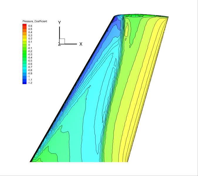
Results are here given for the SU2 solution of inviscid flow over the ONERA M6 wing.

Figure (3): Cp contours on the upper surface of the ONERA M6.

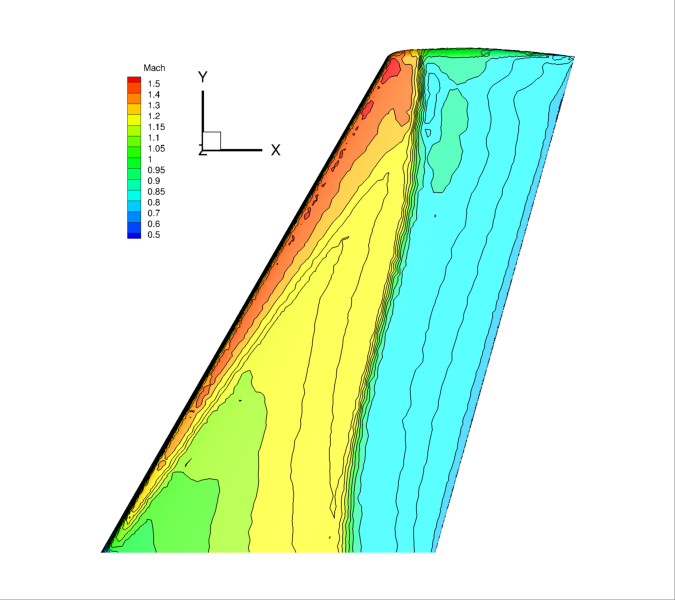Figure (4): Mach number contours on the upper surface of the ONERA M6 wing. Notice the “lambda” shock pattern typically seen on the upper surface.

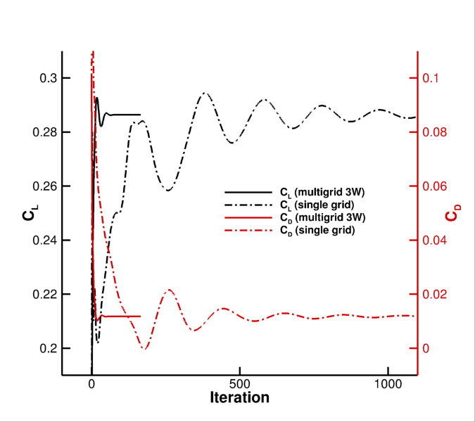Figure (5): Convergence of the non-dimensional coefficients.

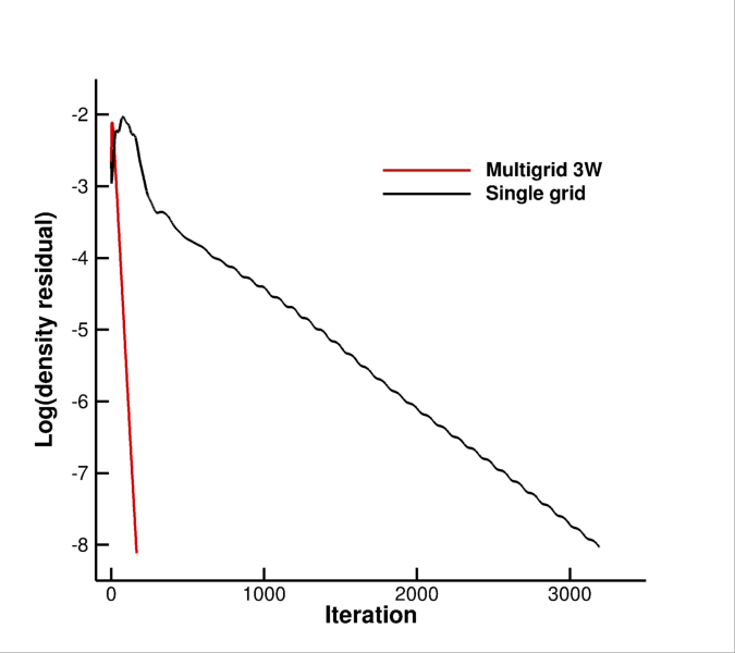Figure (6): Convergence of the density residual (speed up x20, iteration based).