-
Inviscid Bump in a Channel
Inviscid Supersonic Wedge
Inviscid ONERA M6
Laminar Flat Plate
Laminar Cylinder
Turbulent Flat Plate
Transitional Flat Plate
Transitional Flat Plate for T3A and T3A-
Turbulent ONERA M6
Unsteady NACA0012
Epistemic Uncertainty Quantification of RANS predictions of NACA 0012 airfoil
Non-ideal compressible flow in a supersonic nozzle
Non-ideal compressible flows with physics-informed neural networks
Aachen turbine stage with Mixing-plane
-
Inviscid Hydrofoil
Laminar Flat Plate with Heat Transfer
Turbulent Flat Plate
Turbulent NACA 0012
Laminar Backward-facing Step
Laminar Buoyancy-driven Cavity
Streamwise Periodic Flow
Species Transport
Composition-Dependent model for Species Transport equations
Unsteady von Karman vortex shedding
Turbulent Bend with wall functions
Wind velocity and pollutant dispersion in a city
-
Static Fluid-Structure Interaction (FSI)
Dynamic Fluid-Structure Interaction (FSI) using the Python wrapper and a Nastran structural model
Static Conjugate Heat Transfer (CHT)
Unsteady Conjugate Heat Transfer
Solid-to-Solid Conjugate Heat Transfer with Contact Resistance
Incompressible, Laminar counterflow diffusion flame
Incompressible, Laminar Combustion Simulation
User Defined combustion model with Python
-
Unconstrained shape design of a transonic inviscid airfoil at a cte. AoA
Constrained shape design of a transonic turbulent airfoil at a cte. CL
Constrained shape design of a transonic inviscid wing at a cte. CL
Shape Design With Multiple Objectives and Penalty Functions
Unsteady Shape Optimization NACA0012
Unconstrained shape design of a two way mixing channel
Adjoint design optimization of a turbulent 3D pipe bend
Non-linear Elasticity with Multiple Materials
| Written by | for Version | Revised by | Revision date | Revised version |
|---|---|---|---|---|
| @rsanfer | 7.0.2 | @rsanfer | 2020-01-30 | 7.0.2 |
Solver: |
|
Uses: |
|
Prerequisites: |
Non-linear Elasticity |
Complexity: |
Intermediate |
Goals
Once completed the tutorial on Nonlinear Elasticity, we can move on to more advanced features. This document will guide you through the setup of a non-linear problem with multiple material definitions.
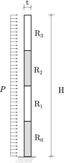
In this tutorial, we use the same problem definition as for the nonlinear elasticity tutorial: a vertical, slender cantilever, clamped in its base, and subject to a horizontal, follower load \(P\) on its left boundary. However, in this section, we will discretize the cantilever into four regions, R0, R1, R2 and R3,
Resources
You can find the resources for this tutorial in the same structural_mechanics/cantilever folder in the Tutorials repository. You can reuse the mesh file mesh_cantilever.su2 from the Non-linear Elasticity tutorial, but you will need a new config file, config_nonlinear_multimaterial.cfg, and an element properties file, element_properties.dat
Background
SU2 has been designed using a finite-deformation framework\(^1\) to account for geometrical and material non-linearities. We can write the non-linear structural problem via the residual equation
\[\mathscr{S}(\mathbf{u}) = \mathbf{T}(\mathbf{u}) - \mathbf{F}_b - \mathbf{F}_{\Gamma}(\mathbf{u})\]which has been obtained from the weak formulation of the structural problem defined using the principle of virtual work and discretized using FEM.
In a Finite Element framework, it is normally possible to define different properties for each element. In this tutorial, we will exemplify the ability of SU2 to deal with this kind of problems.
Configuration File Options
The first thing required to deal with multiple materials, is to add the command
FEA_FILENAME = element_properties.dat
that defines the name of the element-based input file for material definition. This file has the format
INDEX MPROP
0     0
1     0
...
249   0
250   1
...
499   1
500   2
...
749   2
750   3
...
999   3
where the fields, that must be separated by tabs, are:
INDEXcorresponds to the element ID number from the mesh file.MPROPsets the material properties. In this case, the Young’s modulus and the Poisson ratio are:0: \(E\) = 80 GPa, \(\nu\) = 0.41: \(E\) = 10 MPa, \(\nu\) = 0.352: \(E\) = 50 GPa, \(\nu\) = 0.43: \(E\) = 0.5 MPa, \(\nu\) = 0.35
The regions R0, R1, R2 and R3 are assigned the MPROP 0, 1, 2 and 3 respectively, using the config options
ELASTICITY_MODULUS = (8.0E10, 1.0E7, 5.0E10, 5.0E5)
POISSON_RATIO = (0.4, 0.35, 0.4, 0.35)
Finally, given the flexibility of the regions R1 and R3, an incremental approach with 10 increments is adopted.
Running SU2
Follow the links provided to download the config, mesh and element_properties files. Execute the code with the standard command
$ SU2_CFD config_nonlinear_multimaterial.cfg
which will show the following convergence history:
+-----------------------------------------------------------------------------+
|  Inner_Iter|     Load[%]|      rms[U]|      rms[R]|      rms[E]|    VonMises|
+-----------------------------------------------------------------------------+
|           0|     100.00%|   -1.331677|   -0.001635|   -2.028421|  1.0799e+06|
|           1|     100.00%|   -1.913135|    6.972674|    3.447084|  1.0925e+06|

Incremental load: increment 1
+-----------------------------------------------------------------------------+
|  Inner_Iter|     Load[%]|      rms[U]|      rms[R]|      rms[E]|    VonMises|
+-----------------------------------------------------------------------------+
|           0|      10.00%|   -2.331677|   -1.001635|   -4.028421|  1.0799e+05|
|           1|      10.00%|   -3.953012|    5.031711|   -0.519843|  1.0811e+05|
|           2|      10.00%|   -5.865271|    2.061363|   -6.461089|  1.0801e+05|
|           3|      10.00%|   -4.917638|   -1.802157|   -9.113119|  1.0815e+05|
|           4|      10.00%|   -7.297420|    0.015521|  -10.552833|  1.0815e+05|
|           5|      10.00%|   -8.662326|   -5.220135|  -16.527473|  1.0815e+05|
|           6|      10.00%|  -10.815817|   -6.023510|  -20.970444|  1.0815e+05|

...

Incremental load: increment 10
+-----------------------------------------------------------------------------+
|  Inner_Iter|     Load[%]|      rms[U]|      rms[R]|      rms[E]|    VonMises|
+-----------------------------------------------------------------------------+
|           0|     100.00%|   -2.283509|   -0.993242|   -3.982743|  1.0465e+06|
|           1|     100.00%|   -3.756525|    5.121588|   -0.339856|  1.0346e+06|
|           2|     100.00%|   -3.896361|    2.241346|   -6.029630|  1.0345e+06|
|           3|     100.00%|   -3.627203|    1.451203|   -6.004211|  1.0324e+06|
|           4|     100.00%|   -4.983506|    2.651319|   -5.278535|  1.0327e+06|
|           5|     100.00%|   -3.331444|    0.181474|   -5.953341|  1.0275e+06|
|           6|     100.00%|   -4.756347|    3.176148|   -4.231894|  1.0285e+06|
|           7|     100.00%|   -5.265075|   -1.650930|   -9.520310|  1.0285e+06|
|           8|     100.00%|   -6.374912|   -0.472377|  -11.419412|  1.0285e+06|
|           9|     100.00%|   -7.163173|   -2.954409|  -13.740312|  1.0285e+06|
|          10|     100.00%|   -7.779284|   -4.698500|  -14.967597|  1.0285e+06|
|          11|     100.00%|   -8.401311|   -5.725573|  -16.209560|  1.0285e+06|
|          12|     100.00%|   -9.025030|   -5.856932|  -17.456694|  1.0285e+06|
|          13|     100.00%|   -9.649048|   -5.830228|  -18.704672|  1.0285e+06|
|          14|     100.00%|  -10.273113|   -5.868586|  -19.952520|  1.0285e+06|
|          15|     100.00%|  -10.897181|   -5.857269|  -21.195730|  1.0285e+06|
|          16|     100.00%|  -11.521238|   -5.879621|  -22.365896|  1.0285e+06|
|          17|     100.00%|  -12.145524|   -5.909298|  -23.057966|  1.0285e+06|
|          18|     100.00%|  -12.769967|   -5.910878|  -23.152629|  1.0285e+06|
|          19|     100.00%|  -13.393813|   -5.839072|  -23.069515|  1.0285e+06|
The code is stopped as soon as the values of rms[U], rms[R] and rms[E] are below the convergence criteria set in the config file, although for some increments it reaches the maximum number of iterations (20). This is due to the ill conditioning of the matrix of the problem because of the large differences in stiffness between regions.
The displacement field obtained in nonlinear_multimaterial.vtk is shown below:
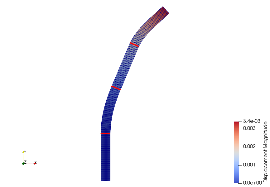
where it can be observed how the flexible regions undergo large deformations, while the regions R0 and R2 remain virtually unaltered due to their high stiffness. The highlighted elements correspond to the interfaces between R1, R2, R3 and R4.
References
\(^1\) Bonet, J. and Wood, R.D. (2008), Nonlinear Continuum Mechanics for Finite Element Analysis, Cambridge University Press
Attribution
If you are using this content for your research, please kindly cite the following reference (reference \(^2\) in the text above) in your derived works:
Sanchez, R. et al. (2018), Coupled Adjoint-Based Sensitivities in Large-Displacement Fluid-Structure Interaction using Algorithmic Differentiation, Int J Numer Meth Engng, Vol 111, Issue 7, pp 1081-1107. DOI: 10.1002/nme.5700
-
This work is licensed under a Creative Commons Attribution 4.0 International License
