Composition-Dependent model for Species Transport equations

Goals

In this tutorial, the user will be familiar with the composition-dependent model in SU2 based on the Ideal Gas law for a gas mixture. The necessary steps and configuration options for the aforementioned model will be explained through a 3D incompressible kenics static mixer for a methane-air mixture.

Resources

The resources for this tutorial can be found in the incompressible_flow/Inc_Species_Transport_Composition_Dependent_Model directory in the tutorial repository. To complete this tutorial, you will need the configuration file (kenics_mixer_tutorial.cfg) and the mesh file (kenics.su2).

The mesh is created using gmsh and a respective .geo script is available to recreate/modify the mesh kenics_mixer_tutorial.geo. The mesh consists of 128790 volume elements and 138324 points.

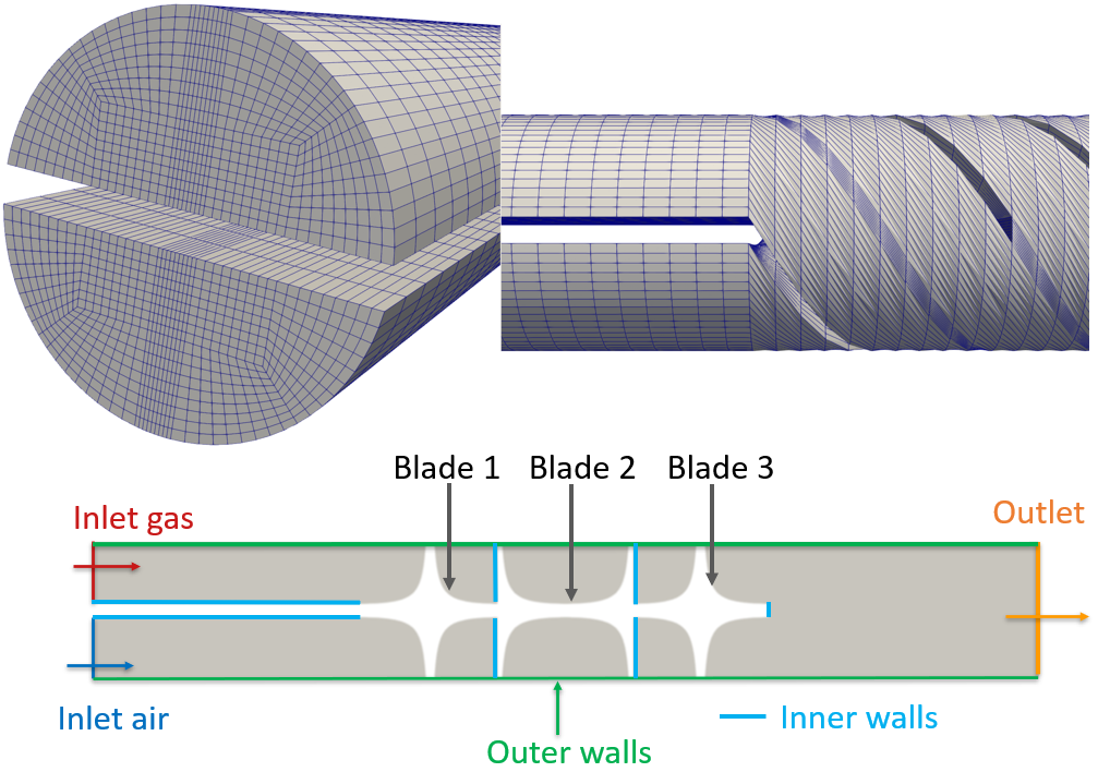Figure (1): Computational mesh (top figure) and 2D cross-section view with color markers showing the boundary conditions and geometry (bottom figure).

Prerequisites

The following tutorial assumes you have already compiled SU2_CFD in serial or parallel, please see the Download and Installation. Likewise, it is advised to perform the tutorial regarding species transport in a venturi mixer(Inc_Species_Transport) where the species transport options are explained, as this tutorial mainly focuses on the composition-dependent options.

Background

The geometry consists of a Static Kenics mixer with three blades, all the blades are perpendicular to each other, and are twisted 180 degrees along the z-axis in order to enhance the mixing. Furthermore, two inlets are considered, where pure air and pure methane are injected at each inlet. Finally, one outlet is considered at the end of the mixer device.

Problem Setup

In this problem, we investigate the flow and mixing along the kenic static mixer. Thus, we have the following boundary conditions at the inlets and outlet:

• Equal Inlet Velocities (constant) = 5 m/s in normal direction (z-direction)
• Outlet Pressure (constant) = 0 Pa
• Inlet Temperature (both inlets) = 300 K
• Adiabatic walls.

In this case, the energy equation is switched OFF as we consider two streams with the same temperature and adiabatic walls.

The SST turbulence model is used with default settings of freestream turbulence intensity of 5% and turbulent-to-laminar viscosity ratio of 10. However, in order to highlight the new option available in SU2 of having different turbulence intensities and turbulent-to-laminar viscosity ratios, these will be given as marker inlets for turbulence that will be explained in the following section.

The thermochemical properties for each gas are given below:

• Methane:
  • Molecular Weight = 16.043 [g / mol]
  • Viscosity: 1.1102E-05 [kg /(m s)]
  • Heat capacity at constant pressure: 2224.43 [J/(kg K)]
  • Thermal Conductivity: 0.0357 [W /(m K)]
• Air:
  • Molecular Weight = 28.960 [g / mol]
  • Viscosity: 1.8551E-05 [kg /(m s)]
  • Heat capacity at constant pressure: 1009.39 [J/(kg K)]
  • Thermal Conductivity: 0.0258 [W /(m K)]

The species mass fractions at each inlet are the following:

• Inlet_gas: mass fraction methane, Y_CH4 = 1.0 (pure methane, Y_air=0.0)
• Inlet_air: mass fraction methane, Y_CH4 = 0.0 (pure air, Y_air=1.0)

It should be noted that within SU2, for a mixture of N species, N-1 species transport equations are solved and, the last species is computed as \(1-\sum Y_i\). Thus, in this tutorial, a transport equation for methane is being solved. For more information, please see Theory.

Configuration File Options

All available options concerning species transport are listed in the config_template.cfg.Here, we are going to focus on the composition-dependent options.

For activating the composition-dependent model, the fluid model must be chosen as FLUID_MODEL= FLUID_MIXTURE. It must be noted that this model is only compatible with INC_DENSITY_MODEL= VARIABLE. Otherwise, an error message will be displayed during runtime.

A low-mach number approximation for incompressible flows allows the pressure to be decomposed into dynamic and thermodynamic (operating) pressure (see Theory. The operating pressure is used for computing the mixture density using the Ideal gas law. The thermodynamic pressure might strongly affect the density at the inlets, causing unphysical results. Therefore, the thermodynamic pressure must be provided by the user for the FLUID_MIXTURE model and, it is no longer computed from the free-stream conditions as it is done in the other fluid models. As in mixing and combustion processes, the operating pressure is often assumed as 101325 pa, then this is the default value considered inside SU2 if the thermodynamic pressure is not given in the .cfg file. In the.cfg file, the thermodynamic pressure is specified as THERMODYNAMIC_PRESSURE= 101325.0.

Subsequently, the molecular weights and heat capacities at constant pressure must be provided as a list as follows: MOLECULAR_WEIGHT= W_1, W_2,...., W_N , SPECIFIC_HEAT_CP = Cp_1, Cp_2,..., Cp_N. The length of the list must match the number of the N species in the mixture. Moreover, the mean molecular weight is computed as a mole fraction average, and the mixture heat capacity is computed as a mass fraction average. For more information, please see \(^{1},^{3}\).

For the conductivity model, the following options are available: CONDUCTIVITY_MODEL= CONSTANT_CONDUCTIVITY, CONSTANT_PRANDTL, POLYNOMIAL_CONDUCTIVITY . In this tutorial, the option CONSTANT_CONDUCTIVITY is used. For this option, a constant conductivity for each species must be provided as follows: THERMAL_CONDUCTIVITY_CONSTANT= k_1, k_2,...., k_N. Currently, the only mixing law available in SU2 for computing the mixture thermal conductivity is based on the Wilke mixing law. Therefore, this is the default option, and it is hardcoded for the FLUID_MIXTURE option. For more information regarding this mixing model, please see \(^{1},^{2}\).

Similar treatment is done for the laminar Prandtl numbers: PRANDTL_LAM= Pr_1, Pr_2,....,Pr_N. Finally, for turbulence simulations, the option of turbulent Prandlt number can be enabled as TURBULENT_CONDUCTIVITY_MODEL= CONSTANT_PRANDTL_TURB. If this option is enabled, the turbulent Prandtl numbers must have the same structure as the Laminar Prandtl numbers: PRANDTL_TURB= Pr_Turb_1, Pr_Turb_2, ..., Pr_Turb_N. For more information about laminar and turbulent Prandlt numbers, please see Theory.

For the present tutorial, the options are given below:

% -------------------- FLUID PROPERTIES ------------------------------------- %
%
FLUID_MODEL= FLUID_MIXTURE
% Thermodynamics(operating) Pressure (101325 Pa default value, only for incompressible flow and FLUID_MIXTURE)
THERMODYNAMIC_PRESSURE= 101325.0
%
MOLECULAR_WEIGHT= 16.043, 28.960
%
SPECIFIC_HEAT_CP = 2224.43, 1009.39
%
CONDUCTIVITY_MODEL= CONSTANT_CONDUCTIVITY
THERMAL_CONDUCTIVITY_CONSTANT= 0.0357, 0.0258
%
PRANDTL_LAM= 0.72, 0.72
%
TURBULENT_CONDUCTIVITY_MODEL= CONSTANT_PRANDTL_TURB
PRANDTL_TURB= 0.90, 0.90

Regarding the viscosity model, the following options are available VISCOSITY_MODEL= SUTHERLAND, CONSTANT_VISCOSITY, POLYNOMIAL_VISCOSITY. In the case of CONSTANT_VISCOSITY, the viscosities must be provided as a list as follows: MU_CONSTANT= mu_1, mu_2, ..., mu_N. Similarly, if SUTHERLAND model is chosen, the Sutherland parameters must be given as a list for each species in the mixture. For completeness, an example for SUTHERLAND option is shown below for a mixture of two species:

% --------------------------- VISCOSITY MODEL ---------------------------------%
%
VISCOSITY_MODEL= SUTHERLAND
% 
MU_REF= 1.118E-05, 1.716E-05
%
MU_T_REF= 273, 273  
%
SUTHERLAND_CONSTANT= 97, 111

For this tutorial, as the energy equation is not being solved, we use CONSTANT_VISCOSITY as the viscosity model. Finally, for computing the mixture viscosity, two models are available in SU2: Wilke and Davidson Models. They can be enabled using the following option: MIXING_VISCOSITY_MODEL = WILKE, DAVIDSON. Please see \(^{2},^{4}\) for more information on these models.. The options used in this tutorial are shown below:

% --------------------------- VISCOSITY MODEL ---------------------------------%
%
VISCOSITY_MODEL= CONSTANT_VISCOSITY
%
MU_CONSTANT= 1.1102E-05, 1.8551E-05 
%
MIXING_VISCOSITY_MODEL = WILKE

The Species transport is switched on by setting KIND_SCALAR_MODEL= SPECIES_TRANSPORT. For the mass diffusivity, the following models are available DIFFUSIVITY_MODEL= CONSTANT_DIFFUSIVITY, CONSTANT_SCHMIDT, UNITY_LEWIS, CONSTANT_LEWIS , where CONSTANT_DIFFUSIVITY is the default model. For the first two, a constant value must be specified in the.cfg file for all species, as it is done in the species transport tutorial Inc_Species_Transport. For the UNITY_LEWIS, no values must be provided because the diffusivity is computed using the mixture thermal conductivity, density and heat capacity at constant pressure; for more information, please see \(^{3}\). For highly diffusive gases, such as hydrogen, the CONSTANT_LEWIS option could be used. For this option, the Lewis numbers of the N-1 species for which a transport equation is being solved must be provided as a list using the option CONSTANT_LEWIS_NUMBER= Le_1, Le_2, ..., Le_N_1. Finally, for turbulent simulations, the turbulent diffusivity is computed based on the SCHMIDT_NUMBER_TURBULENT. For reference, please consult the respective theory.

Finally, for the SST model, it is possible to provide the intensity and turbulent-to-laminar viscosity ratios per inlet. For this option, we use the following structure: MARKER_INLET_TURBULENT= (inlet_1, TurbIntensity_1, TurbLamViscRatio_1, inlet_2, TurbIntensity_2, TurbLamViscRatio_2, ...).

As final remarks, the option MARKER_SPECIES_STRONG_BC is advised to not to be used when the convective scheme for species and turbulent are CONV_NUM_METHOD_SPECIES= BOUNDED_SCALAR and CONV_NUM_METHOD_TURB= BOUNDED_SCALAR, respectively. When SCALAR_UPWIND is used in both cases, the MARKER_SPECIES_STRONG_BC is advised to be used to enforce boundary conditions and improve convergence for this convective scheme. This can be used with the following structure MARKER_SPECIES_STRONG_BC= (marker1, marker2, ....). The convective scheme BOUNDED_SCALAR will be further explained in the section Convective-Schemes.

Likewise, SPECIES_CLIPPING= NO is only recommended when the option SCALAR_UPWIND is used. The option BOUNDED_SCALAR performs well without using the clipping option.

The other species transport options can be found in the species transport tutorial(Inc_Species_Transport).

For completeness, the options aforementioned are shown below:

% -------------------- BOUNDARY CONDITION DEFINITION --------------------------%
%
MARKER_HEATFLUX= ( inner_wall, 0.0,blade_1, 0.0, blade_2, 0.0, blade_3, 0.0, outer_wall,0.0)
%
SPECIFIED_INLET_PROFILE= NO
%
INC_INLET_TYPE=  VELOCITY_INLET VELOCITY_INLET
MARKER_INLET= ( inlet_gas, 300, 5.0, 0.0,  0.0, 1.0, inlet_air, 300, 5.0, 0.0, 0.0, 1.0 )
MARKER_INLET_SPECIES= (inlet_gas, 1.0, inlet_air, 0.0 )
%
MARKER_INLET_TURBULENT= (inlet_gas, 0.05, 10, inlet_air, 0.05, 10)
INC_OUTLET_TYPE= PRESSURE_OUTLET
MARKER_OUTLET= ( outlet, 0.0 )
%
% --------------------- SPECIES TRANSPORT SIMULATION --------------------------%
%
% Specify scalar transport model (NONE, SPECIES_TRANSPORT)
KIND_SCALAR_MODEL= SPECIES_TRANSPORT
%
% Mass diffusivity model (CONSTANT_DIFFUSIVITY)
DIFFUSIVITY_MODEL= UNITY_LEWIS
%
% Turbulent Schmidt number of mass diffusion
SCHMIDT_NUMBER_TURBULENT= 0.7
%
% Convective numerical method for species transport (SCALAR_UPWIND, BOUNDED_SCALAR)
CONV_NUM_METHOD_SPECIES= BOUNDED_SCALAR
%
% Monotonic Upwind Scheme for Conservation Laws (TVD) in the species equations.
% Required for 2nd order upwind schemes (NO, YES)
MUSCL_SPECIES= NO
%
% Slope limiter for species equations (NONE, VENKATAKRISHNAN, VENKATAKRISHNAN_WANG, BARTH_JESPERSEN, VAN_ALBADA_EDGE)
SLOPE_LIMITER_SPECIES = NONE
%
% Time discretization for species equations (EULER_IMPLICIT, EULER_EXPLICIT)
TIME_DISCRE_SPECIES= EULER_IMPLICIT
%
% Initial values for scalar transport
SPECIES_INIT= 1.0
%
% Activate clipping for scalar transport equations
SPECIES_CLIPPING= NO

Running SU2

The simulation can be run in serial using the following command:

$ SU2_CFD kenics_mixer_tutorial.cfg

or in parallel with your preferred number of cores (for this case, it is recommended to use 4 cores in order to speed up the simulation):

$ mpirun -n <#cores> SU2_CFD kenics_mixer_tutorial.cfg

Results

This case shows a smooth convergence and does not have the flat residuals observed in the Inc_Species_Transport.

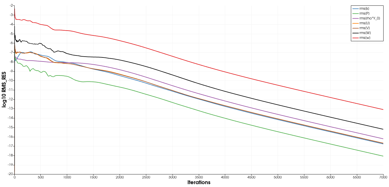Figure (2): Residual plot (Incompressible mean flow, SST turbulence model, species transport).

We observe that using the option CONV_NUM_METHOD_SPECIES= BOUNDED_SCALAR addressed the unphysical mass fraction fluctuations observed in the tutorial (Inc_Species_Transport). Similarly, it can be noted how the mixing process is enhanced by the mixer units.

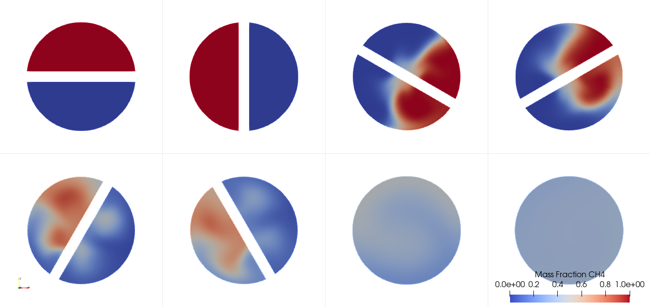Figure (3): Mass fractions of methane at the different locations along the Kenics static mixer.

Velocity magnitude along the Kenics static mixers.

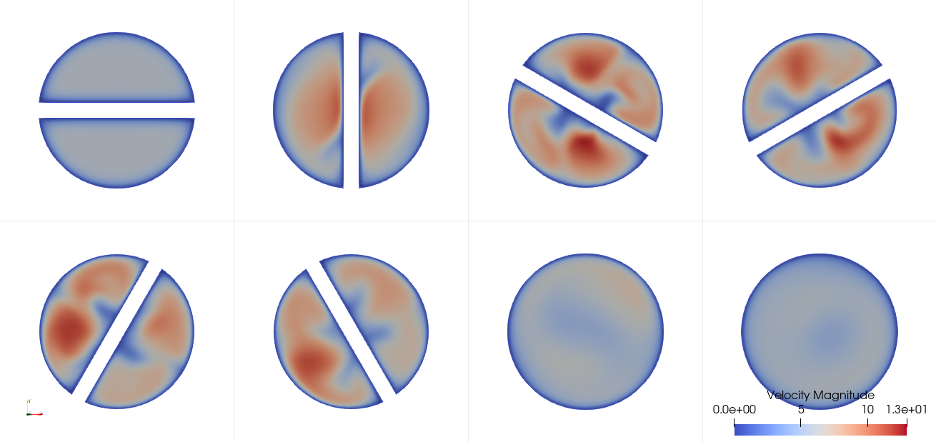Figure (4): Velocity magnitude at different locations along the Kenics static mixer.

The plots are cross sections of the mixing device at the following locations: 0.04, 0.09, 0.1067, 0.1133, 0.1267, 0.1333, 0.18 and 0.24 m.

References

\(^{1}\) B. Poling, J. Prausnitz, J. O’Connell, The Properties of Gases and Liquids, 5th Edition, McGraw-Hill Education,2000.(URL https://books.google.nl/books?id=9tGclC3ZRX0C)

\(^{2}\) C. R. Wilke, A viscosity equation for gas mixtures, The Journal of Chemical Physics 18 (4) (1950),517–519.(https:doi:10.1063/1.1747673).

\(^{3}\) T. Poinsot, D. Veynante, Theoretical and Numerical Combustion, Ch. 1, 2012.

\(^{4}\) T. A. Davidson, A simple and accurate method for calculating viscosity of gaseous mixtures. (URL https://www.osti.gov/biblio/6129940)

Additional remarks