-
Inviscid Bump in a Channel
Inviscid Supersonic Wedge
Inviscid ONERA M6
Laminar Flat Plate
Laminar Cylinder
Turbulent Flat Plate
Transitional Flat Plate
Transitional Flat Plate for T3A and T3A-
Turbulent ONERA M6
Unsteady NACA0012
Epistemic Uncertainty Quantification of RANS predictions of NACA 0012 airfoil
Non-ideal compressible flow in a supersonic nozzle
Non-ideal compressible flows with physics-informed neural networks
Aachen turbine stage with Mixing-plane
-
Inviscid Hydrofoil
Laminar Flat Plate with Heat Transfer
Turbulent Flat Plate
Turbulent NACA 0012
Laminar Backward-facing Step
Laminar Buoyancy-driven Cavity
Streamwise Periodic Flow
Species Transport
Composition-Dependent model for Species Transport equations
Unsteady von Karman vortex shedding
Turbulent Bend with wall functions
Wind velocity and pollutant dispersion in a city
-
Static Fluid-Structure Interaction (FSI)
Dynamic Fluid-Structure Interaction (FSI) using the Python wrapper and a Nastran structural model
Static Conjugate Heat Transfer (CHT)
Unsteady Conjugate Heat Transfer
Solid-to-Solid Conjugate Heat Transfer with Contact Resistance
Incompressible, Laminar Combustion Simulation
User Defined combustion model with Python
-
Unconstrained shape design of a transonic inviscid airfoil at a cte. AoA
Constrained shape design of a transonic turbulent airfoil at a cte. CL
Constrained shape design of a transonic inviscid wing at a cte. CL
Shape Design With Multiple Objectives and Penalty Functions
Unsteady Shape Optimization NACA0012
Unconstrained shape design of a two way mixing channel
Adjoint design optimization of a turbulent 3D pipe bend
Non-linear Elasticity
| Written by | for Version | Revised by | Revision date | Revised version |
|---|---|---|---|---|
| @rsanfer | 7.0.2 | @rsanfer | 2020-01-28 | 7.0.2 |
Solver: |
|
Uses: |
|
Prerequisites: |
Linear Elasticity |
Complexity: |
Intermediate |
Goals
Once completed the tutorial on Linear Elasticity, we can move on to non-linear problems. This document will guide you throught the following capabilities of SU2:
- Setting up a non-linear structural problem with large deformations
- Non-linear (hyperelastic) material law
- Follower boundary conditions
- Incremental loads
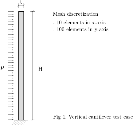
In this tutorial, we use the same problem definition as for the linear elastic case: a vertical, slender cantilever, clamped in its base, and subject to a horizontal, follower load \(P\) on its left boundary. This is shown in Fig. 1.
Resources
You can find the resources for this tutorial in the same structural_mechanics/cantilever folder in the Tutorials repository. You can reuse the mesh file mesh_cantilever.su2 from the Linear Elasticity tutorial, but you will need a new config file, config_nonlinear.cfg.
Background
SU2 has been designed using a finite-deformation framework\(^1\) to account for geometrical and material non-linearities.
We can write the non-linear structural problem via the residual equation
\[\mathscr{S}(\mathbf{u}) = \mathbf{T}(\mathbf{u}) - \mathbf{F}_b - \mathbf{F}_{\Gamma}(\mathbf{u})\]which has been obtained from the weak formulation of the structural problem defined using the principle of virtual work and discretized using FEM. The state variable \(\mathbf{u}\) corresponds to the displacements of the structure with respect to its reference configuration \(\mathbf{R}\). \(\mathbf{T}(\mathbf{u})\) are the internal equivalent forces, \(\mathbf{F}_b\) are the body forces and \(\mathbf{F}_{\Gamma}(\mathbf{u})\) are the surface forces applied over the external boundaries of the structure.
We can linearize the structural equation as
\[\mathscr{S}(\mathbf{u}) + \frac{\partial \mathscr{S}(\mathbf{u})}{\partial \mathbf{u}} \Delta \mathbf{u} = \mathbf{0}\]where the tangent matrix is \(\mathbf{K} = \partial \mathscr{S}(\mathbf{u})/\partial \mathbf{u}\). The linearized problem is solved using a Newton method until convergence. Further description of the approach adopted in SU2 can be found in a paper by Sanchez et al\(^2\).
Mesh Description
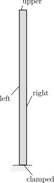
The cantilever is discretized using 1000 4-node quad elements with linear interpolation. The boundaries are defined as follows:
Configuration File Options
We start the tutorial by definining the structural properties. In this case, we will solve a geometrically non-linear problem, with a Neo-Hookean material model.
GEOMETRIC_CONDITIONS= LARGE_DEFORMATIONS
MATERIAL_MODEL= NEO_HOOKEAN
We adopt a plane strain formulation for the 2D problem, and reduce the stiffness of the cantilever by 2 orders of magnitude as compared to the Linear Elasticity tutorial, so that the beam undergoes large deformations:
ELASTICITY_MODULUS=5E7
POISSON_RATIO=0.35
FORMULATION_ELASTICITY_2D = PLANE_STRAIN
Now, we define the Newton-Raphson strategy to solve the non-linear problem. We set the solution method and maximum number of subiterations using
NONLINEAR_FEM_SOLUTION_METHOD = NEWTON_RAPHSON
INNER_ITER = 15
Then, the convergence criteria is set to evaluate the norm of the displacement vector (RMS_UTOL), the residual vector (RMS_RTOL) and the energy (RMS_ETOL). We set the convergence values to -8.0, which is the log10 of the previously defined magnitudes.
CONV_FIELD= RMS_UTOL, RMS_RTOL, RMS_ETOL
CONV_RESIDUAL_MINVAL= -8,
Finally, we define the boundary conditions. In this case, the load applied to the left boundary will be an uniform, follower pressure, that is, its direction will change with the changes in the normals of the surface. This is done as
MARKER_CLAMPED = ( clamped )
MARKER_PRESSURE = ( left, 1E3, upper, 0, right, 0)
Running SU2
Follow the links provided to download the config and mesh files. Execute the code with the standard command
$ SU2_CFD config_nonlinear.cfg
which will show the following convergence history:
+----------------------------------------------------------------+
|  Inner_Iter|      rms[U]|      rms[R]|      rms[E]|    VonMises|
+----------------------------------------------------------------+
|           0|   -1.454599|   -0.001635|   -2.082200|  1.1259e+06|
|           1|   -2.406133|    3.664361|   -0.038068|  1.1224e+06|
|           2|   -3.623182|    2.288350|   -2.827362|  1.1053e+06|
|           3|   -3.096627|   -0.433125|   -5.369087|  1.1229e+06|
|           4|   -4.547761|    0.493533|   -6.401479|  1.1222e+06|
|           5|   -5.306858|   -2.420278|   -9.740703|  1.1221e+06|
|           6|   -6.878854|   -3.854770|  -12.877010|  1.1221e+06|
|           7|   -8.478641|   -6.065417|  -16.078409|  1.1221e+06|
|           8|  -10.081222|   -7.667567|  -19.283559|  1.1221e+06|
|           9|  -11.683669|   -8.697378|  -22.488189|  1.1221e+06|
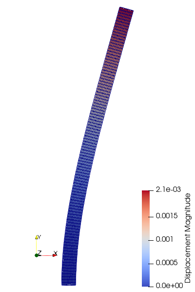
The code is stopped as soon as the values of rms[U], rms[R] and rms[E] are below the convergence criteria set in the config file. The displacement field obtained in nonlinear.vtk is shown below:
Increasing the load
The magnitude of the residual can limit the convergence of the solver, particularly for those cases in which the problem is very non-linear. Say, for example, that we multiply the load in the left boundary by 4, using
MARKER_PRESSURE = ( left, 4E3, upper, 0, right, 0)
Running SU2 now would result in the divergence of the solver,
+----------------------------------------------------------------+
|  Inner_Iter|      rms[U]|      rms[R]|      rms[E]|    VonMises|
+----------------------------------------------------------------+
|           0|   -0.852539|    0.600425|   -0.878080|  4.5753e+06|
|           1|   -1.130461|    4.628370|    2.207826|  4.4618e+06|
|           2|   -2.198592|    4.658260|    1.539054|  2.8742e+08|
|           3|        -nan|        -nan|        -nan|  0.0000e+00|
|           4|        -nan|        -nan|        -nan|  0.0000e+00|
due to a large imbalance between the internal and external loads. It can be observed that the order of magnitude of the residual vector grows above 104. To solve this problem, we have incorporated an incremental approach to SU2, that applies the load in linear steps,
\[\mathbf{F}_i = \frac{i}{N}\mathbf{F}\]where \(i\) is the step and \(N\) the maximum number of increments allowed. To apply the load in increments, we need to use the following commands
INCREMENTAL_LOAD = YES
NUMBER_INCREMENTS = 25
INCREMENTAL_CRITERIA = (2.0, 2.0, 2.0)
where \(N\) = 25, and the criteria to apply the increments is that either one of rms[U] > 2.0, rms[R] > 2.0 or rms[E] > 2.0 is met. We add an option to print out the load increment to the screen output:
SCREEN_OUTPUT = (INNER_ITER, LOAD_INCREMENT, RMS_UTOL, RMS_RTOL, RMS_ETOL, VMS)
If we now run the code,
+-----------------------------------------------------------------------------+
|  Inner_Iter|     Load[%]|      rms[U]|      rms[R]|      rms[E]|    VonMises|
+-----------------------------------------------------------------------------+
|           0|     100.00%|   -0.852539|    0.600425|   -0.878080|  4.5753e+06|
|           1|     100.00%|   -1.130461|    4.628370|    2.207826|  4.4618e+06|

Incremental load: increment 1
+-----------------------------------------------------------------------------+
|  Inner_Iter|     Load[%]|      rms[U]|      rms[R]|      rms[E]|    VonMises|
+-----------------------------------------------------------------------------+
|           0|       4.00%|   -2.250479|   -0.797515|   -3.673960|  1.7944e+05|
|           1|       4.00%|   -4.005792|    2.096002|   -3.207727|  1.7948e+05|
|           2|       4.00%|   -5.555428|   -0.881184|   -9.113457|  1.7949e+05|
|           3|       4.00%|   -7.611025|   -4.228316|  -14.254076|  1.7949e+05|
|           4|       4.00%|  -10.343696|   -7.532184|  -19.528442|  1.7949e+05|
|           5|       4.00%|  -13.138042|   -8.791438|  -24.949847|  1.7949e+05|
given that 4.628370 > 2.0 and 2.207826 > 2.0, the load is applied in \(\Delta \mathbf{F} = 1/25 \mathbf{F}\), completing the simulation in the 25th step,
Incremental load: increment 25
+-----------------------------------------------------------------------------+
|  Inner_Iter|     Load[%]|      rms[U]|      rms[R]|      rms[E]|    VonMises|
+-----------------------------------------------------------------------------+
|           0|     100.00%|   -2.188244|   -0.786306|   -3.616397|  4.2701e+06|
|           1|     100.00%|   -3.417010|    2.241142|   -2.911125|  4.2325e+06|
|           2|     100.00%|   -2.802795|   -0.383540|   -4.853108|  4.1931e+06|
|           3|     100.00%|   -3.461966|    1.059169|   -5.203155|  4.2102e+06|
|           4|     100.00%|   -4.053497|   -0.412173|   -7.024221|  4.2103e+06|
|           5|     100.00%|   -4.505028|   -1.211625|   -8.188042|  4.2090e+06|
|           6|     100.00%|   -5.044900|   -2.434771|   -9.288963|  4.2093e+06|
|           7|     100.00%|   -5.572267|   -3.418852|  -10.345812|  4.2092e+06|
|           8|     100.00%|   -6.099258|   -4.140827|  -11.400141|  4.2093e+06|
|           9|     100.00%|   -6.625915|   -4.693663|  -12.453409|  4.2093e+06|
|          10|     100.00%|   -7.152645|   -5.224056|  -13.506885|  4.2093e+06|
|          11|     100.00%|   -7.679350|   -5.750731|  -14.560291|  4.2093e+06|
|          12|     100.00%|   -8.206063|   -6.277523|  -15.613718|  4.2093e+06|
|          13|     100.00%|   -8.732773|   -6.804154|  -16.667138|  4.2093e+06|
|          14|     100.00%|   -9.259484|   -7.329682|  -17.720560|  4.2093e+06|
|          15|     100.00%|   -9.786195|   -7.846390|  -18.773983|  4.2093e+06|
|          16|     100.00%|  -10.312907|   -8.293905|  -19.827405|  4.2093e+06|
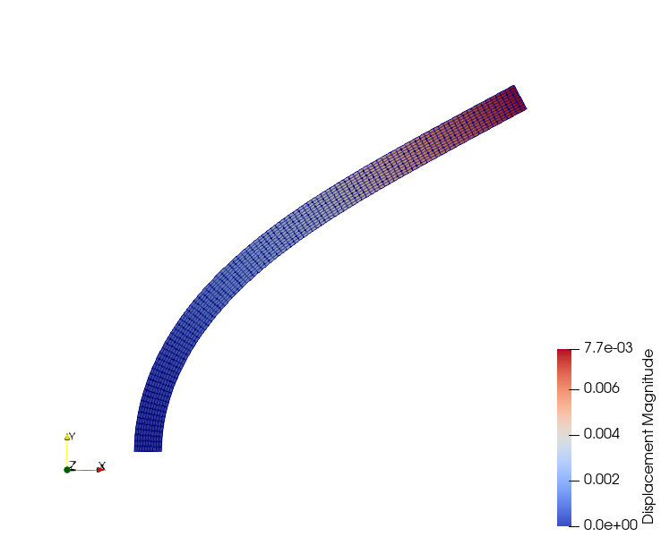
The displacement field is now
References
\(^1\) Bonet, J. and Wood, R.D. (2008), Nonlinear Continuum Mechanics for Finite Element Analysis, Cambridge University Press
Attribution
If you are using this content for your research, please kindly cite the following reference (reference \(^2\) in the text above) in your derived works:
Sanchez, R. et al. (2018), Coupled Adjoint-Based Sensitivities in Large-Displacement Fluid-Structure Interaction using Algorithmic Differentiation, Int J Numer Meth Engng, Vol 111, Issue 7, pp 1081-1107. DOI: 10.1002/nme.5700
-
This work is licensed under a Creative Commons Attribution 4.0 International License
