Dynamic Fluid-Structure Interaction (FSI) using the Python wrapper and a Nastran structural model

Goals

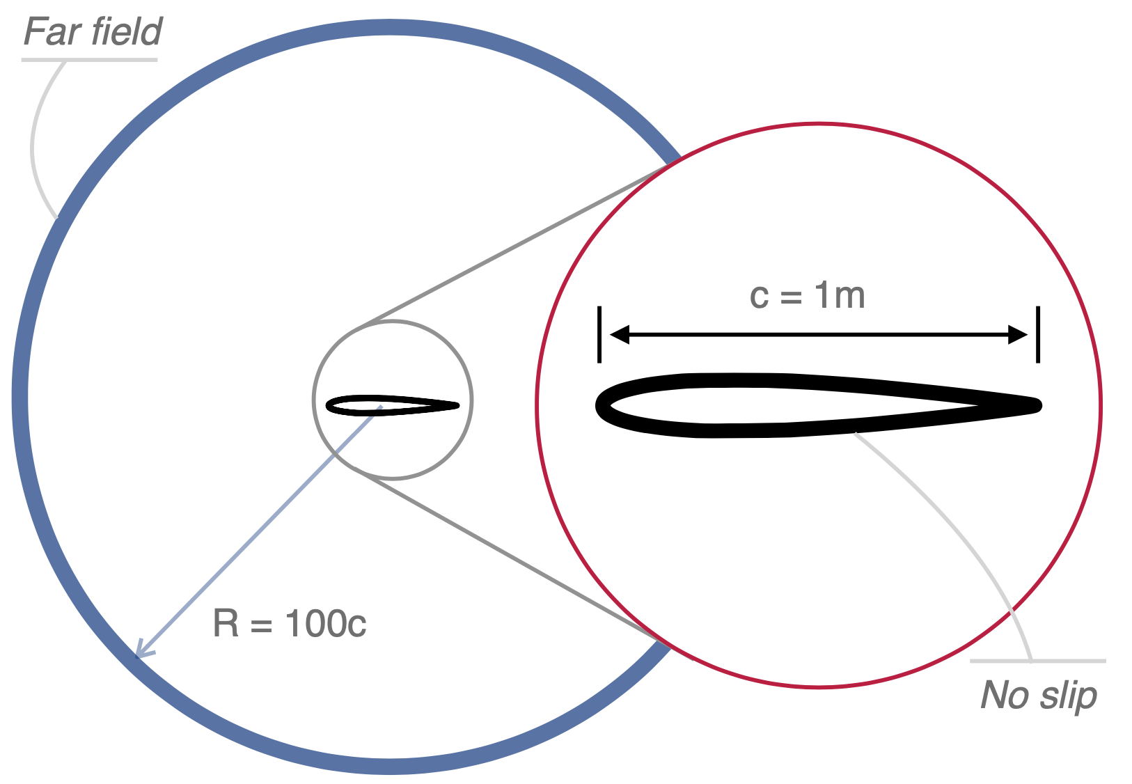
This tutorial shows how to exploit the capabilities of the Python wrapper to couple SU2 with an external structural solver. The problem at hand consists in a NACA 0012 airfoil, free to pitch and plunge, with given stiffnesses, immersed in a flow with varying Mach number. The two frequencies of the modes of the structure will vary as the speed is increased, reaching a point when the aeroelastic system will be unstable. The classical pitch-plunge flutter will then be visible.

The considered case has been presented in \(^1\), the reader is encouraged to refer to that reference for further details on the problem.

The structual solver used in this example couples SU2 with the commercial code Nastran, keeping the results of general interest. Indeed, linear strctures of arbitrary complexity can be analysed with the same workflow.

Summarizing, this document will cover:

• Preparing a FSI analysis to be used with the python wrapper
• Using the structural solver for Nastran models with SU2
• Important keywords for the fsi and solid solver config files

A sketch of the problem at hand is presented below:

Resources

You can find the resources for this tutorial in this folder of the Tutorials repository. There is a matlab file that can be used to produce validation data with Theodorsen theory and the mesh file.

In the main directory, there are other 5 subdirectories containing the configuration files and structural models for the different Mach numbers. Please do not mix those files as the structural models and configurations are different at the different aerodynamic conditions.

Before starting this tutorial, please be sure to have compiled SU2 with the python wrapper enabled. Further, two packages are required that can be downloaded from your package manager: libspatialindex and petsc, with their python counterparts rtree and petsc4py.

Background

The solution process will follow a very similar flow as the one explained in this tutorial, which you should complete before stepping to the present one. The fluid and structural solutions will be obtained separately, iterating between them until convergence. Here, the difference is due to the fact that the simulation is unsteady. Thus, this inner iteration between fluid and struture will be repeated at each physical time step.

The aerodynamic model is based on the compressible Reynolds-averaged Navier-Stokes equations. A central JST scheme is used for the convective fluxes, and a weighted least square scheme is used for the gradients. The turbulence model is the SST and a CFL number of 20, for the psuedo time step, is used.

Different Mach numbers will be considered, namely \(Ma=[0.1, 0.2, 0.3, 0.357, 0.364]\). The Reynolds number is fixed at 4 millions, and the temperature is equal to 273K.

The structural model is made by a single point, positioned at the rotation axis, with two degrees of freedom, pitch and plunge. Inertia and mass of the airfoil are concentrated at the center of mass of the profile, at a certain distance from the rotation axis. The equations of motions are available analytically and read:

Where \(m\) is the mass of the airfoil, \(I\) the inertia around the rotation axis, \(S\) the static moment of inertia at the rotation axis, \(C\) and \(K\) the dampings and stiffnesses respectively. \(L\) and \(M\) are the lift and pitching up moment.

These equations are usually adimensionalised to obtain results independent from the free-stream density of the flow. Indeed, we can define the following parameters:

\(\chi=\frac{S}{mb}\), \(r_{\alpha}^2=\frac{I_f}{mb^2}\), \(\bar{\omega}=\frac{\omega_h}{\omega_{\alpha}}\), \(\mu=\frac{m}{\pi \rho_{\infty} b^2}\)

Where \(b\) is the semi chord of the airfoil, \(\omega_h = \sqrt{\frac{K_h}{m}}\) \(\omega_{\alpha} = \sqrt{\frac{K_{\alpha}}{I_f}}\). If we fix them, the structure will behave always the same regardless of \(\rho_{\infty}\).

In this context \(\chi=0.25\), \(r_{\alpha}=0.5\), \(\omega_{\alpha} = 45 rad/s\), \(\bar{\omega}=0.3185\) and \(\mu=100\).

Note that, as we will vary the Mach number, the density will also change accordingly. Thus, with given nondimensional parameters, the inertias and stiffnesses must be varied accordingly.

No structural damping is included and a time step of 1ms is used.

The structural solver, instead of integrating the equations of motions for this point, which are available analytically, is intended to solve a general structural problem. For this reason, a preprocessing step in Nastran will be performed, computing the mode shapes and modal frequencies of the model. Then, the structural solver will integrate a set of ODEs for the modes of the structure.

To perform the preprocessing step, in the case control section of the Nastran model (i.e. at the very beginning of the file), the following lines must be added:

• ECHO = SORT
• DISPLACEMENT(PRINT,PUNCH)=ALL

A real egeinvalue analysis will then be performed. This will produce, in the f06 file, an equivalent, ordered, model that will eventually be read by the python script to create the interface. Further, it will be created a punch file where all the mode shapes, together with modal stiffnesses, are stored.

IMPORTANT: The modes should be normalised to unit mass.

Further, in the Nastran model, a SET1 card must be added that contains all the nodes to be interfaced with aerodynamics. Note that, as of now, only one SET1 card is allowed. However, this should be sufficiently general not to create issues.

The input and output reference systems of the interface nodes can be defined as local, but these reference systems must be directly defined with respect to the global one. Thus, if node x is referring to reference system y, y must be defined with respect to the global one.

In the structural input file the keyword NMODES must then be defined to select which, of all the modes in the punch file, to be used.

In this particular case, it may look excessively complicated, but it allows to solve an arbitrary aeroelastic problem with the same scheme.

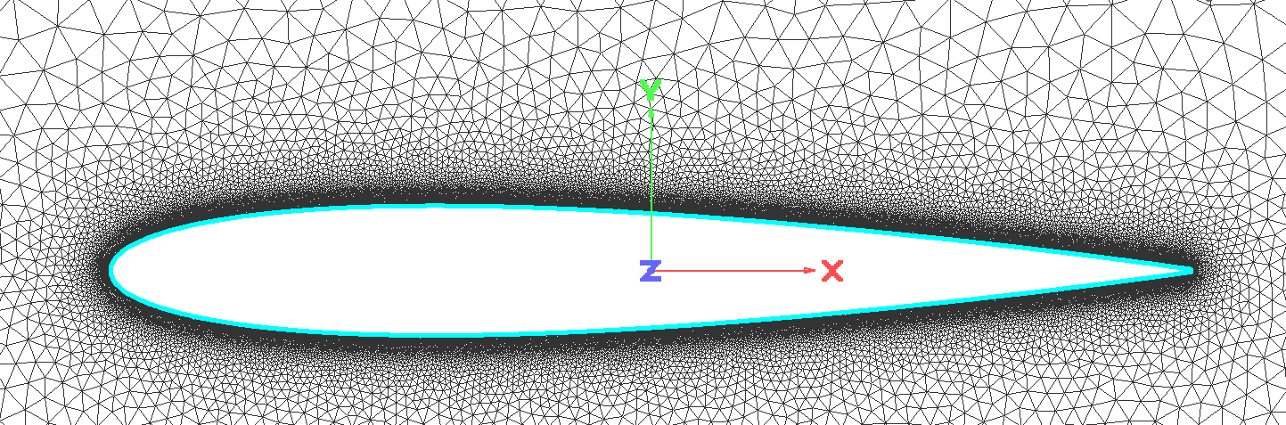
Mesh Description

The fluid domain is discretised with 133k nodes, with refining close to the airfoil surface, in order to correctly represent the turbulent boundary layer. The first cell is placed at a height of \(y+\approx 1\). A close up view of the mesh is pictured below:

As far as the structural mesh is concerned, this is a finite element mesh prepared for the commercial code Nastran. In the context of this example, as only a 2D problem, with only two degrees of freedom, is considered, the mesh is extremely simple; a set of rigid elements that connect several slave nodes to the only master node, positioned on the rotation axis. The master node only has two degrees of freedom: pitch and plunge.

One of the slave nodes, at the position of the center of mass, houses the mass and inertia of the airfoil.

It should always be recalled that, if interpolation is needed between the structural and fluid meshes, RBF will be used. The limitation of this linear interpolation is due to the fact that, if a 2D problem is concerned, the structural points cannot all lie on the same line. Equivalently, if a 3D problem is tackled, the points cannot lie all in the same plane. For this reason, the thickness is represented in the FEM mesh for Nastran as shown below:

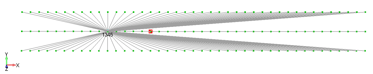
As you can see, the exact profile is not required. The interpolation will take care of displacing correctly the fluid mesh. However, thickness must somehow be represented.

Configuration File for the fluid zone

First of all, the users should know that three configuration files are required for this case: one for the fluid zone, one for the solid zone and one for the interface. The configuration file for the fluid zone is very similar to a configuration file for a simple single zone simulation. Indeed, SU2 does not know about the external structural solver, it will only see the points on the aerodynamic mesh changing positions.

For this reason, the solver keyword is set as:

SOLVER = RANS

A new marker is introduced, MARKER_DEFORM_MESH_SYM_PLANE. This marker is effectively a symmetry marker for the mesh deformation only. It may be useful in cases where symmetry in the mesh is required, but not in the fluid simulation. An example may be the simulation of a plane half-model, in wind tunnel, where the effect of boundary layer on the tunnel walls must be studied, but a pitch movement of the model is also allowed. Fluid symmetry cannot be used, but at the same time the mesh should move on the tunnel wall to match the deformation given by the pitch motion. However, in the context of this example, this marker is not required.

The only difference from a common single zone configuration file is the addition of the following lines:

%-------------- Coupling conditions -------------------------------------------%
DEFORM_MESH = YES
MARKER_DEFORM_MESH = ( airfoil )
DEFORM_STIFFNESS_TYPE = WALL_DISTANCE
DEFORM_LINEAR_SOLVER_ITER= 200

Where we selected the airfoil as our marker for coupling.

The simulation is unsteady with a physical time step of 1ms:

TIME_DOMAIN = YES
TIME_STEP= 1e-3

It is important to set an appropriate convergence criteria for the fluid zone. Indeed, while the structural part is linear and requires no iterations, it is important that the fluid zone correctly converges for accurate results.

The relative residual cannot be used as this is reset at each inner iteration. Thus, after the first inner loop, it would be difficult to obtain convergence as the absolute residuals are already quite low. For this reason we will use:

CONV_CRITERIA = RESIDUAL
CONV_FIELD= RMS_DENSITY
CONV_RESIDUAL_MINVAL= -9.0

Configuration File for the solid zone

This configuration file will be read by the structural python solver included in SU2, that will read the preprocessed Nastran model.

The solver can work in two ways:

1. It can impose the movement of a mode, with prescribed law, to provide forced response analysis

2. It can integrate in time the modal equations of motion to study the linearised structural deformations when the body is surrounded by the flow

Available keywords for the config file:

• NMODES (int): number of modes to use in the analysis. If n modes are available in the punch file, but only the first m<n are required, set this to m

• RESTART_ITER (int): if restart is used, this specifies the iteration to restart

• DELTA_T (float): physical time step size to be used in the simulation. Must match the one in SU2

• MODAL_DAMPING (float): the code is able to add a damping matrix to the system, based on a critical damping. This keyword specifies the amount of damping that can be included: if x% of damping is required, set it to 0.0x

• RHO (float): rho parameter for the integrator

• TIME_MARCHING (string): YES or NO

• MESH_FILE (string): path to the f06 file

• PUNCH_FILE (string): path to the pch file

• RESTART_SOL (string): YES or NO

• MOVING_MARKER (string): numerical ID of the SET1 card indentifying the group of nodes to be used as interface

• IMPOSED_MODES (dictionary): In case of imposed motion this list contains the modes with imposed motion and the type of motion. Example: IMPOSED_MODES={0:["SINUSOIDAL"],3:["BLENDED_STEP"],4:["SINUSOIDAL"]}. If more imposed motions have to be superposed on the same mode, we can write: IMPOSED_MODES={0:["SINUSOIDAL","BLENDED_STEP"]}

• IMPOSED_PARAMETERS (dictionary): Depending on what was selected above, different parameters are required to complete the definition of motion. For example, in case of a sinusoidal motion, it is required to know if there is a bias, the initial time, the frequency and the amplitude. If we want to specify a sine with no bias, initial time of 5s, 20 of amplitude and 10 Hz of frequency for mode 7, we would write: IMPOSED_PARAMETERS={6:[{"BIAS":0.0, "AMPLITUDE":20.0, "FREQUENCY":10.0, "TIME_0":5.0}]}. Please note that more imposed motions can be superposed on the same mode simply adding more entries for the same mode: IMPOSED_PARAMETERS={6:[{...},{...}]}. For more information about these parameters please look at the module pysu2_nastran.py. Note that the order of the parameter dictionaries must be coincident with the order defined in IMPOSED_MODES dictionary.

• INITIAL_MODES (dictionary): list containing the initial amplitudes of the modes. Example is {0:0.1,1:0.0,3:5.0,…}

We will call the Nastran model modal.bdf and, after the eigenvalue analysis, we will obtain the files modal.f06 and modal.pch.

In the context of our problem, the configuration file will read:

NMODES = 2
MESH_FILE = modal.f06
PUNCH_FILE = modal.pch
MOVING_MARKER = airfoil
TIME_MARCHING = YES
RESTART_SOL = NO
MODAL_DAMPING = 0.0
DELTA_T = 0.001
RHO = 0.5
% 5 degrees of pitch and no plunge
INITIAL_MODES = {0:-0.1061,1:-0.1657}

The modes are coupled. Thus, appropriate initial conditions, to obtain 5 degrees of pitch and no plunge, must be obtained from the mode amplitudes at the master node.

Configuration File for the interface

The most important interface configuration keywords are:

• NDIM (int): 2 or 3 depending if the model is bidimensional or tridimensional

• RESTART_ITER (int): Restart iteration

• TIME_TRESHOLD (int): Time iteration after which fluid and structure are coupled in an unsteady simulation

• NB_FSI_ITER (int): Number of max internal iterations to couple fluid and structure

• RBF_RADIUS (float): Radius for the RBF interpolation. It is dimensional (i.e. in meters) and must be set so that at least 5 structural points are always inside a sphere with that radius and centered in any of the structural nodes. The more nodes are included, the better the interpolation. However, with a larger radius, the interpolation matrix becames less sparse and the solution more computationally expensive

• AITKEN_PARAM (float): Under relaxation parameter, between 0 and 1

• UNST_TIMESTEP (float): Physical time step size in unsteady simulations, must match the one in the other cfg files

• UNST_TIME (float): Physical simulation time for unsteady problems

• FSI_TOLERANCE (float): Tolerance for inner loop convergence between fluid and structure. This is the maximum average structural displacements, between two inner iterations, that can be accepted

• CFD_CONFIG_FILE_NAME (string): Path to the fluid cfg file

• CSD_SOLVER (string): Structural solver to be used. As of now, only the native modal solver is used, activated with the keyword NATIVE. However, other solvers can easily be added

• IMPOSED_MOTION (string): YES or NO. Specifies wether the structural solver will integrate the structural equations or just impose a specific movement. In the latter case, forces are not mapped onto the structure, as it would not be required.

• MAPPING_MODES (string): YES or NO. Special feature that can only be used with the native solver. Used to extract the mapped modes onto the aerodynamic mesh.

• CSD_CONFIG_FILE_NAME (string): Path to the solid cfg file

• RESTART_SOL (string): YES or NO

• MATCHING_MESH (string): YES or NO, the fluid and structural mesh match at the interface

• MESH_INTERP_METHOD (string): Interpolation method in case of nonmatching meshes. TPS or RBF

• DISP_PRED (string): Displacement predictor order FIRST_ORDER or SECOND_ORDER. To be used in unsteady simulations

• AITKEN_RELAX (string): DYNAMIC or STATIC

• TIME_MARCHING (string): YES or NO

NDIM = 2
NB_FSI_ITER = 20
RBF_RADIUS = 0.5
AITKEN_PARAM = 0.4
UNST_TIMESTEP = 0.001
UNST_TIME = 4.0
TIME_TRESHOLD = 99
FSI_TOLERANCE = 0.000001
CFD_CONFIG_FILE_NAME = fluid.cfg
CSD_SOLVER  = AEROELASTIC
CSD_CONFIG_FILE_NAME = solid.cfg
RESTART_SOL = NO
MATCHING_MESH = NO
MESH_INTERP_METHOD = RBF
DISP_PRED = SECOND_ORDER
AITKEN_RELAX = DYNAMIC
TIME_MARCHING = YES

Running SU2

Follow the links provided to download the main directory.

The preprocessing step in Nastran has already been performed, thus you will directly find the required structural model.

Copy the mesh file in each subdirectory, then run the following command from inside each subdirectory:

$ python3 /your/path/to/fsi_computation.py -f fsi.cfg

If you built you version of SU2 in parallel, run instead:

$ mpirun -np X python3 -m mpi4py /your/path/to/fsi_computation.py --parallel -f fsi.cfg

Substituting X with the appropriate number of cores. The -m flag set to mpi4py will instruct python to call MPI_Abort() in case of unhandled exceptions. In this way, you will avoid reaching deadlocks during execution.

You will see, after the usual preprocessing steps, the following output:

**********************************
* Begin unsteady FSI computation *
**********************************

Setting FSI initial conditions
Checking f/s interface conservation...
Solid side (Wx, Wy, Wz) = (0.0, 0.0, 0.0)
Fluid side (Wx, Wy, Wz) = (0.0, 0.0, 0.0)

Performing static mesh deformation (ALE) of initial mesh...


FSI initial conditions are set
Beginning time integration

In these steps, an initial deformation is imposed, if required, and the mesh is deformed accordingly. Afterwards, the computation can start:

>>>> Time iteration 0 / FSI iteration 0 <<<<
Checking f/s interface conservation...
Solid side (Wx, Wy, Wz) = (0.0, 0.0, 0.0)
Fluid side (Wx, Wy, Wz) = (0.0, 0.0, 0.0)

Performing dynamic mesh deformation (ALE)...

CSysSolve::FGMRES(): system solved by initial guess.

Launching fluid solver for one single dual-time iteration...
+-----------------------------------------------------------------------------+
|   Time_Iter|  Inner_Iter|          CD|          CL|    rms[Rho]| relrms[Rho]|
+-----------------------------------------------------------------------------+
|           0|           0|    2.925114|   -5.650014|   -2.772504|    0.000000|
|           0|           1|    2.419387|   -4.707503|   -3.257713|   -0.485209|
|           0|           2|    2.039722|   -3.799496|   -3.346967|   -0.574463|
|           0|           3|    1.887042|   -3.439476|   -3.470247|   -0.697743|
|           0|           4|    1.831439|   -3.346855|   -3.558842|   -0.786338|
|           0|           5|    1.800010|   -3.330105|   -3.595711|   -0.823207|
|           0|           6|    1.769099|   -3.325896|   -3.588726|   -0.816222|
|           0|           7|    1.732970|   -3.321408|   -3.551232|   -0.778728|

This is the typical output that you will see. There was no initial deformation imposed and for this reason you can see that the mesh deformation system was solved by the initial guess. FSI iteration is the inner iteration index, and it will keep increasing until the inner convergence is found. Then, this index will be set to zero and the time iteration will be increased.

Please do not confuse Inner_Iter with FSI iteration. The former is the iteration, in the fluid zone only, using the pseudo time; the latter is the iteration index between fluid and structure.

After all the computations are completed (i.e. for all the Mach numbers), in each case folder you will see a file called StructHistoryModal.dat. The first rows of this file, for Mach number 0.1, are reported below.

Time	Time Iteration  FSI Iteration       q1          qdot1   qddot1  q2      qdot2  qddot2	
0.099	99	            1	            -0.1501	0.0000  30.0116	-0.2343	0.0000 649.9362	
0.100	100	            2	            -0.1500	0.0505  66.9711	-0.2339	0.6319 617.5777	
0.101	101	            1	            -0.1499	0.1133  63.2111	-0.2330	1.2470 609.8225	
0.102	102                 1               -0.1498     0.1754  60.8115	-0.2314	1.8549 605.5686	
0.103	103	            1	            -0.1496	0.2352  58.7621	-0.2293	2.4576 599.9707	
0.104	104	            1	            -0.1493	0.2931  56.9690	-0.2265	3.0535 592.1878	
0.105	105	            1	            -0.1490	0.3493  55.3371	-0.2232	3.6407 582.3177	

The first column contains the physical time (please note that we started the fluid-structure coupling after 99 time iterations), the second one contains the time iteration, the third one the number of FSI iterations required for convergence, then we have the time histories of the modes and their derivatives.

For many applications this may be already the desired output. However, in this case, we actually want the physical rotation and displacement of the point at the rotation axis. A post processing step must be performed to multiply the mode shapes for their amplitude. This can be done with the provided matlab file. You only need to run the Main_compare.m file and it will take care of all the required operations.

Please note that those files are absolutely general. Thus, feel free to reuse them for other models.

At the end of the matlab run, you will see outputs as the ones reported below.

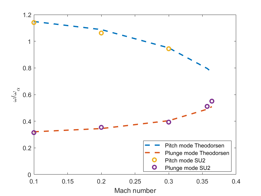
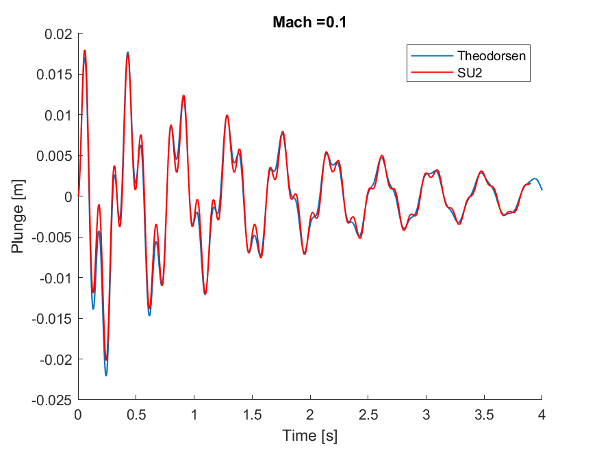
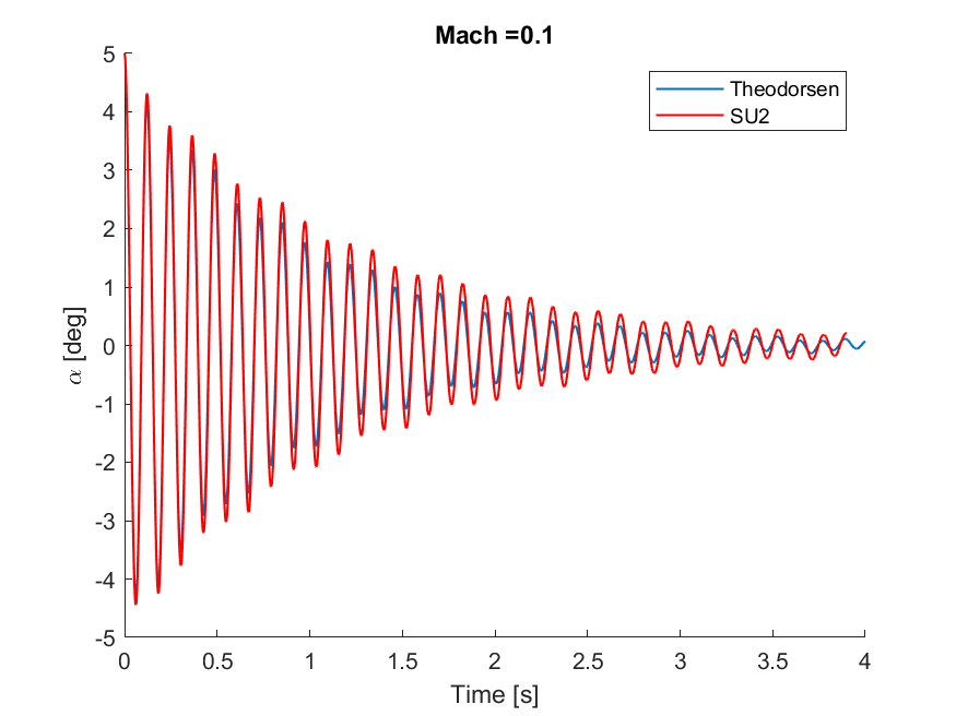
You can see how the frequency merging is well captured; after the flutter point the two frequencies are coincident and nonlinear effects are present. Thus, comparing the Theodorsen theory and SU2 is not fully meaningful. The time histories also match nicely.

References

\(^1\) Sanchez, R. (2018), A coupled adjoint method for optimal design in fluid-structure interaction problems with large displacements, PhD thesis, Imperial College London, DOI: 10.25560/58882

Attribution

Fonzi, N., Cavalieri, V., De Gaspari, A., & Ricci, S. (2022). Extended computational capabilities for high-fidelity fluid-structure simulations, Journal of Computational Science, Vol. 62, July 2022, 101698. Link to publication

This work is licensed under a Creative Commons Attribution 4.0 International License