Species Transport

Goals

Upon completing this tutorial, the user will be familiar with adding passive species transport equations to an incompressible or compressible flow problem. The necessary steps and config options will be explained with the example of a simple 2D incompressible mixing channel system. Output options will be explained as well.

Limitations: Mixture dependent fluid properties are not available yet. The mass diffusion coefficient can only be chosen as a constant for a all species transport equations.

Resources

The resources for this tutorial can be found in the incompressible_flow/Inc_Species_Transport directory in the tutorial repository. You will need the configuration file (species3_primitiveVenturi.cfg) and the mesh file (primitiveVenturi.su2).

The mesh is created using gmsh and a respective .geo script is available to recreate/modify the mesh primitiveVenturi.geo. The mesh is fully structured (i.e. only contains Quadrilateral elements) with 3364 elements and 3510 points. A progression towards walls is used but the mesh resolution is for demonstration purposes only. The small size also makes it ideal for code development.

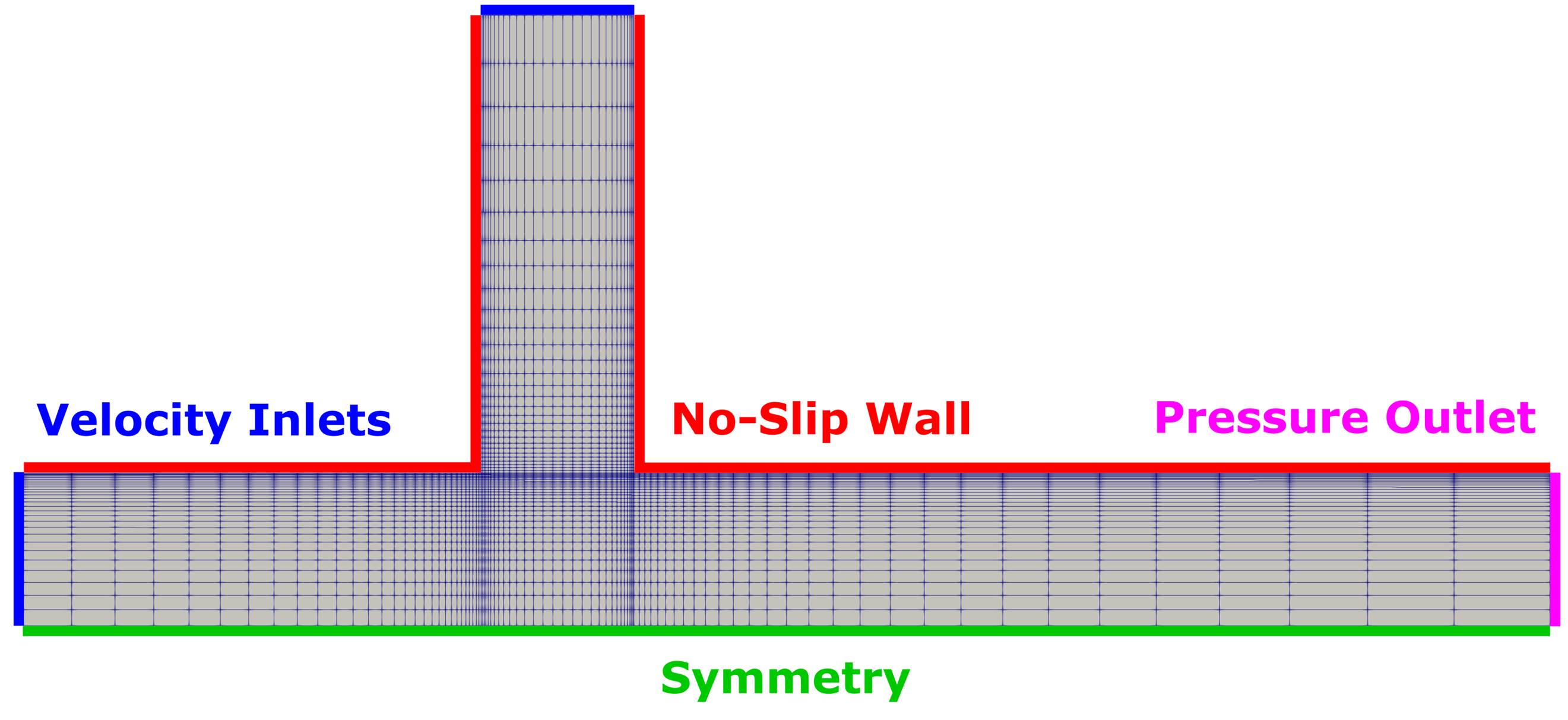Figure (1): Computational mesh with color indication of the used boundary conditions.

Prerequisites

The following tutorial assumes you already compiled SU2_CFD in serial or parallel, please see the Download and Installation if that is not done yet. Additionally it is advised to perform an entry level incompressible tutorial first, as this tutorial only goes over species transport

Background

The geometry with two separate inlets, a junction where the two feeders meet and a nozzle leading to an outlet, resembles loosely a venturi mixer. The geometry massively simplifies these design principles. The material properties and provided mass fractions at the inlet are for demonstration purposes.

Problem Setup

The material properties of the incompressible mean flow represent air:

• Density (constant) = 1.1766 kg/m^3
• Viscosity (constant) = 1.716e-5 kg/(m-s)
• Inlet Velocities (constant) = 1 m/s in normal direction
• Outlet Pressure (constant) = 0 Pa

The SST turbulence model is used with the default settings of freestream turbulence intensity of 5% and a turbulent-to-laminar viscosity ratio of 10.

The material properties specific to the species transport equations are:

• Mass Diffusivity (constant) = 1e-3 m^2/s
• Mass fractions at the eastern inlet: 0.5, 0.5
• Mass fractions at the northern inlet: 0.6, 0.0

Configuration File Options

All available options concerning species transport are listed below as they occur in the config_template.cfg.

The options as of now are fairly limited. Species transport is switched on by setting KIND_SCALAR_MODEL= SPECIES_TRANSPORT. The DIFFUSIVITY_MODEL= CONSTANT_DIFFUSIVITY is currently the only available therefore the only additional choice the value of DIFFUSIVITY_CONSTANT. For the SCHMIDT_NUMBER_TURBULENT please consult the respective theory.

The number of species transport equations is not set individually but deduced from the number of values given in the respective lists for species options. SU2 checks whether the same amount of values is given in each option and solves the appropriate amount of equations. MARKER_INLET_SPECIES is one of these options and has to be used alongside a usual MARKER_INLET. For outlets, symmetries or walls this is not necessary.

The option SPECIES_USE_STRONG_BC should be left to NO and is an experimental option where a switch to strongly enforced boundary conditions can be made.

For CONV_NUM_METHOD_SPECIES= SCALAR_UPWIND a second order MUSCL reconstruction and multiple limiters are available.

The TIME_DISCRE_SPECIES can be either an implicit or explicit euler and a CFL reduction coefficient CFL_REDUCTION_SPECIES compared to the regular CFL_NUMBER is available.

The inital species mass fractions are given by the list SPECIES_INIT= 1.0, ....

SPECIES_CLIPPING= YES with the respective lists for min and max enforces a strict lower and upper limit for the mass fraction solution used by the solver.

% --------------------- SPECIES TRANSPORT SIMULATION --------------------------%
%
% Specify scalar transport model (NONE, SPECIES_TRANSPORT)
KIND_SCALAR_MODEL= SPECIES_TRANSPORT
%
% Mass diffusivity model (CONSTANT_DIFFUSIVITY)
DIFFUSIVITY_MODEL= CONSTANT_DIFFUSIVITY
%
% Mass diffusivity if DIFFUSIVITY_MODEL= CONSTANT_DIFFUSIVITY is chosen. D_air ~= 0.001
DIFFUSIVITY_CONSTANT= 0.001
%
% Turbulent Schmidt number of mass diffusion
SCHMIDT_NUMBER_TURBULENT= 0.7
%
% Inlet Species boundary marker(s) with the following format:
% (inlet_marker, Species1, Species2, ..., SpeciesN-1, inlet_marker2, Species1, Species2, ...)
MARKER_INLET_SPECIES= (inlet, 0.5, ..., inlet2, 0.6, ...)
%
% Use strong inlet and outlet BC in the species solver
SPECIES_USE_STRONG_BC= NO
%
% Convective numerical method for species transport (SCALAR_UPWIND)
CONV_NUM_METHOD_SPECIES= SCALAR_UPWIND
%
% Monotonic Upwind Scheme for Conservation Laws (TVD) in the species equations.
% Required for 2nd order upwind schemes (NO, YES)
MUSCL_SPECIES= NO
%
% Slope limiter for species equations (NONE, VENKATAKRISHNAN, VENKATAKRISHNAN_WANG, BARTH_JESPERSEN, VAN_ALBADA_EDGE)
SLOPE_LIMITER_SPECIES = NONE
%
% Time discretization for species equations (EULER_IMPLICIT, EULER_EXPLICIT)
TIME_DISCRE_SPECIES= EULER_IMPLICIT
%
% Reduction factor of the CFL coefficient in the species problem
CFL_REDUCTION_SPECIES= 1.0
%
% Initial values for scalar transport
SPECIES_INIT= 1.0, ...
%
% Activate clipping for scalar transport equations
SPECIES_CLIPPING= NO
%
% Maximum values for scalar clipping
SPECIES_CLIPPING_MAX= 1.0, ...
%
% Minimum values for scalar clipping
SPECIES_CLIPPING_MIN= 0.0, ...

For the screen, history and volume output multiple straight forward options were included. Whenever a number is used at the end of the keyword, one for each species (starting at zero) can be added.

SCREEN_OUTPUT= RMS_SPECIES_0, ..., MAX_SPECIES_0, ..., BGS_SPECIES_0, ..., \
               LINSOL_ITER_SPECIES, LINSOL_RESIDUAL_SPECIES, \
               SURFACE_SPECIES_0, ..., SURFACE_SPECIES_VARIANCE

For HISTORY_OUTPUT the residuals are included in RMS_RES and the linear solver quantities in LINSOL. The surface outputs can be included with SPECIES_COEFF or SPECIES_COEFF_SURF for each surface individually.

For VOLUME_OUTPUT no extra output field has the be set. The mass fractions are included in SOLUTION and the volume residuals in RESIDUAL.

All available output can be printed to screen using the dry-run feature of SU2:

$ SU2_CFD -d <config-filename>.cfg

Running SU2

The simulation can be run in serial using the following command:

$ SU2_CFD species3_primitiveVenturi.cfg

or in parallel with your preferred number of cores (for this small case not more than 4 cores should be used):

$ mpirun -n <#cores> SU2_CFD species3_primitiveVenturi.cfg

Results

The case converges nicely as expected on such a simple case and mesh.

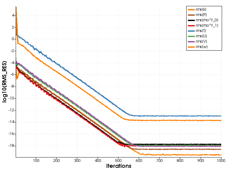Figure (2): Residual plot (Incompressible mean flow, SST turbulence model, species transport).

Note that there is still some unphysical mass fraction fluctuation for Species_0 at the junction corner. This becomes much less apparent by using MUSCL_SPECIES = YES but does not fully disappear.

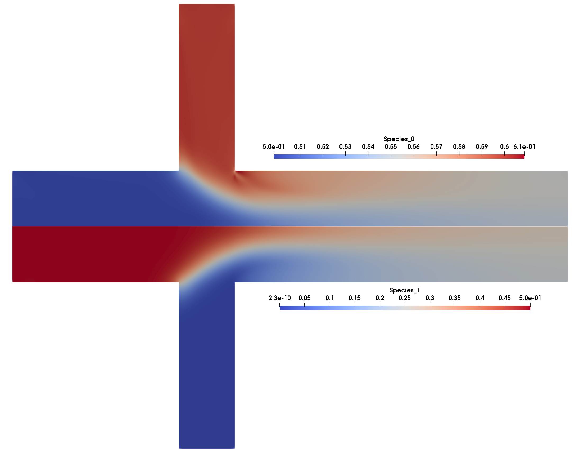Figure (3): Volume mass fractions for both species. Species_1 is mirrored for better comparison.

Velocity magnitude field along which the species are transported. For a much less homogenous mixture at the outlet one could decrease the DIFFUSIVITY_CONSTANT which makes for a more interesting optimization problem.

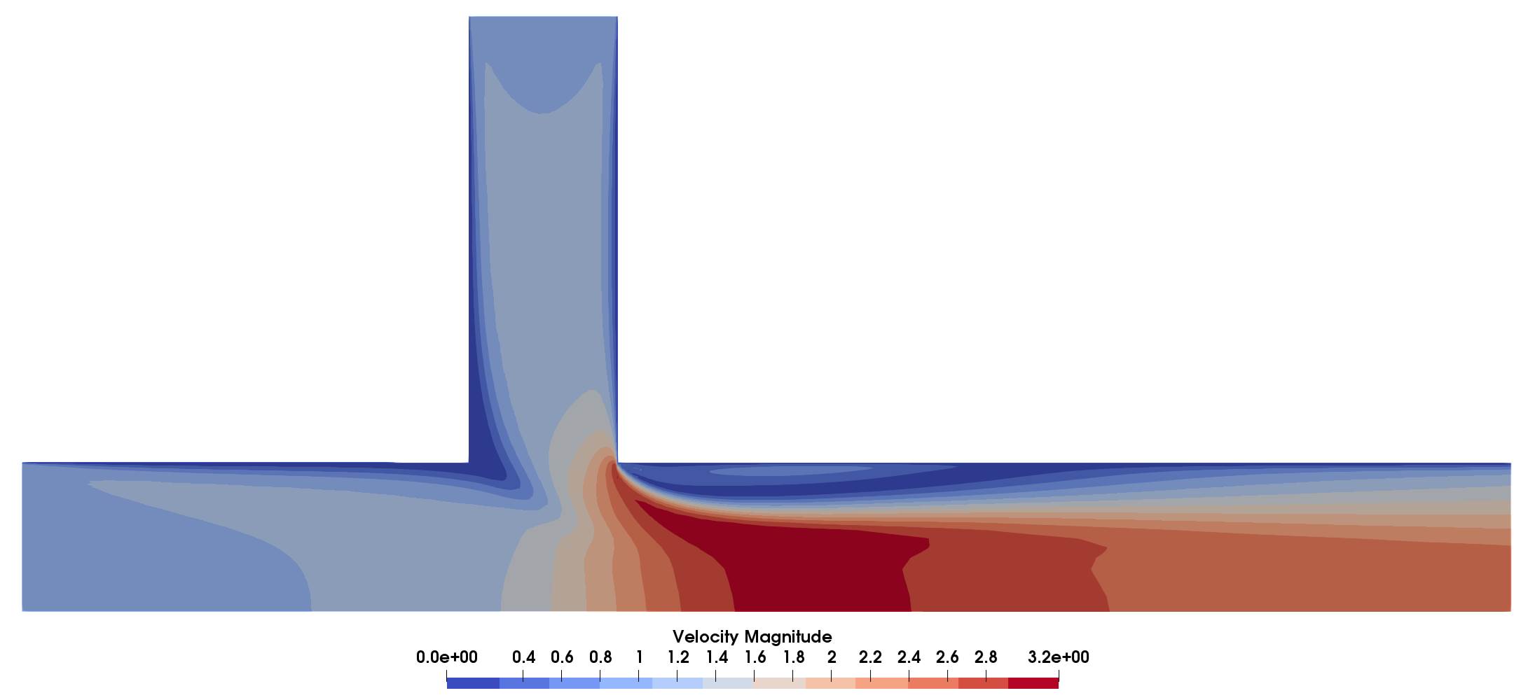Figure (4): Velocity Magnitude in the domain.

Additional remarks

An in depth optimization of this case with addition of the FFD-box, gradient validation and some more steps can found here.