Linear Dynamics

Goals

Upon completion of the tutorial on Linear Elasticity, this document will guide you throught the following capabilities of SU2:

• Setting up a dynamic structural problem with small deformations
• Time-dependent boundary conditions
• Newmark integration method

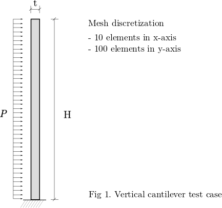
The problem that we will be solving consists of a vertical, slender cantilever, clamped in its base, and subject to a horizontal, time-dependent load \(P\) on its left boundary. This is shown in Fig. 1.

Resources

For this tutorial, it is assumed that you have first completed the guide on Linear Elasticity guide. You can find the resources for this tutorial in the same structural_mechanics/cantilever folder in the Tutorials repository. You can reuse the mesh file mesh_cantilever.su2 but need a new config file, config_dynamic.cfg.

Background

This tutorial covers the solution of structural dynamics problems. The equation of the problem is now

\(\mathbf{M}\mathbf{\ddot{u}}+\mathbf{K}\mathbf{u}=\mathbf{F}\),

where \(\mathbf{K}\) and \(\mathbf{K}\) are respectively the stiffness and mass matrices of the cantilever, \(\mathbf{u}\) is the vector of displacements of the structural nodes, \(\mathbf{\ddot{u}}\) is the vector of accelerations of the structural nodes, and \(\mathbf{F}\) is the vector of applied forces, and the structural damping effects have been neglected.

This tutorial will be solved the for the cantilever with the following conditions:

• Young’s modulus: \(\mathrm{E = 5.0}\) \(\mathrm{GPa}\)
• Poisson ratio: \(\nu\) \(\mathrm{= 0.35}\)
• Solid density: \(\rho\) \(\mathrm{= 1000}\) \(\mathrm{kg/m^3}\)
• Height: \(\mathrm{H = 10}\) \(\mathrm{mm}\)
• Thickness: \(\mathrm{t = 0.5}\) \(\mathrm{mm}\)

Mesh Description

The cantilever is discretized using 1000 4-node quad elements with linear interpolation. The boundaries are defined as follows:

Configuration File Options

We start from the configuration options used on the tutorial on [Linear Elasticity]. However, for this case set the analysis to be dynamic using

TIME_DOMAIN = YES
TIME_STEP = 0.01
TIME_ITER = 250

where the time step \(\Delta t\) has been set to 10 ms, and the total time of the simulation is \(T = 2.5\) s (250 time steps). We will be using the Newmark\(^1\) method for time integration, which relies on the approximations

and

to advance the problem in time. Further details about the implementation can be found on this reference by Sanchez et al\(^2\), available for download at Spiral.

We will be introducing a 2% numerical damping, to damp out higher frequencies in the problem. This is done by setting

TIME_DISCRE_FEA = NEWMARK_IMPLICIT
NEWMARK_BETA = 0.2601
NEWMARK_GAMMA = 0.52

We maintain the structural properties from the previous example. In dynamic problems, inertial effects are incorporated throught the mass matrix \(\mathbf{M}\). Therefore, it is necessary to define the density of the material, which is done through the following option,

MATERIAL_DENSITY = 1000

Finally, we define a sinusoidal load, \(\mathrm{P}(t) = A \sin(2\pi f t+\phi)\mathrm{P}\), being \(f\) the frequency of the sine wave in Hz, \(A\) the amplitude and \(\phi\) the phase angle in rad. This introduces some dynamic effects into the problem. We do so using

SINE_LOAD = YES
SINE_LOAD_COEFF = (1.5, 2.0, 4.7124)

where SINE_LOAD_COEFF= (\(A\), \(f\), \(\phi\)). We have set a phase angle \(\phi = -3\pi/2\) and an amplitude \(A = 1.5\), which leads to a load \(P(t) = -1.5P = -1.5 \textrm{kPa}\) at time \(t=0\). The frequency is \(f=2\) Hz, which leads to 5 full cycles of oscillation in our time span \(T = 5\) s.

Running SU2

This is a very small example that we can run in serial. To run this test case, follow these steps at a terminal command line:

1. Move to the directory containing the config file (config_dynamic.cfg) and the mesh file (mesh_cantilever.su2). Make sure that the SU2 tools were compiled, installed, and that their install location was added to your path.

2. Run the executable by entering

   $ SU2_CFD config_dynamic.cfg
   

   at the command line.

3. SU2 will print the residual of the linear solver for each time step, and the simulation will finish after 250 time steps.
4. Files containing the results will be written upon exiting SU2. The flow solution can be visualized in ParaView (.vtk) or Tecplot (.dat for ASCII).

For this particular problem, the solver should have run very quickly. Please note, a large number of files (500) will be generated upon running SU2 for this case, 2 files corresponding for each time step.

The screen output of the code will go over your settings, before initializing the solver. Once done so, you will obtain an output to screen such as

+---------------------------------------------------+
|   Time_Iter|  rms[DispX]|  rms[DispY]|    VonMises|
+---------------------------------------------------+
|         249|  -11.145342|  -11.309566|  1.7175e+06|

----------------------------- Solver Exit -------------------------------
Maximum number of time iterations reached (TIME_ITER = 250).
-------------------------------------------------------------------------
+-----------------------------------------------------------------------+
|        File Writing Summary       |              Filename             |
+-----------------------------------------------------------------------+
|SU2 restart                        |restart_linear_dynamic_00249.dat   |
|Paraview binary                    |linear_dynamic_00249.vtk           |
+-----------------------------------------------------------------------+

where rms[DispX] and rms[DispY] correspond to the residual of the linear solver in the x and y components of the displacements, and VonMises corresponds to the maximum Von Mises Stress in the structural domain.

Results

The output files append the time step as linear_dynamic__*****.vtk. They contain the displacement field, the nodal tensions \(\sigma_{xx}\), \(\sigma_{yy}\) and \(\sigma_{xy}\) (as Sxx, Syy and Sxy), and the Von Misses stress. In order to visualize the deformation of the cantilever on Paraview, one can use the filter Warp By Vector applied on the displacement field.

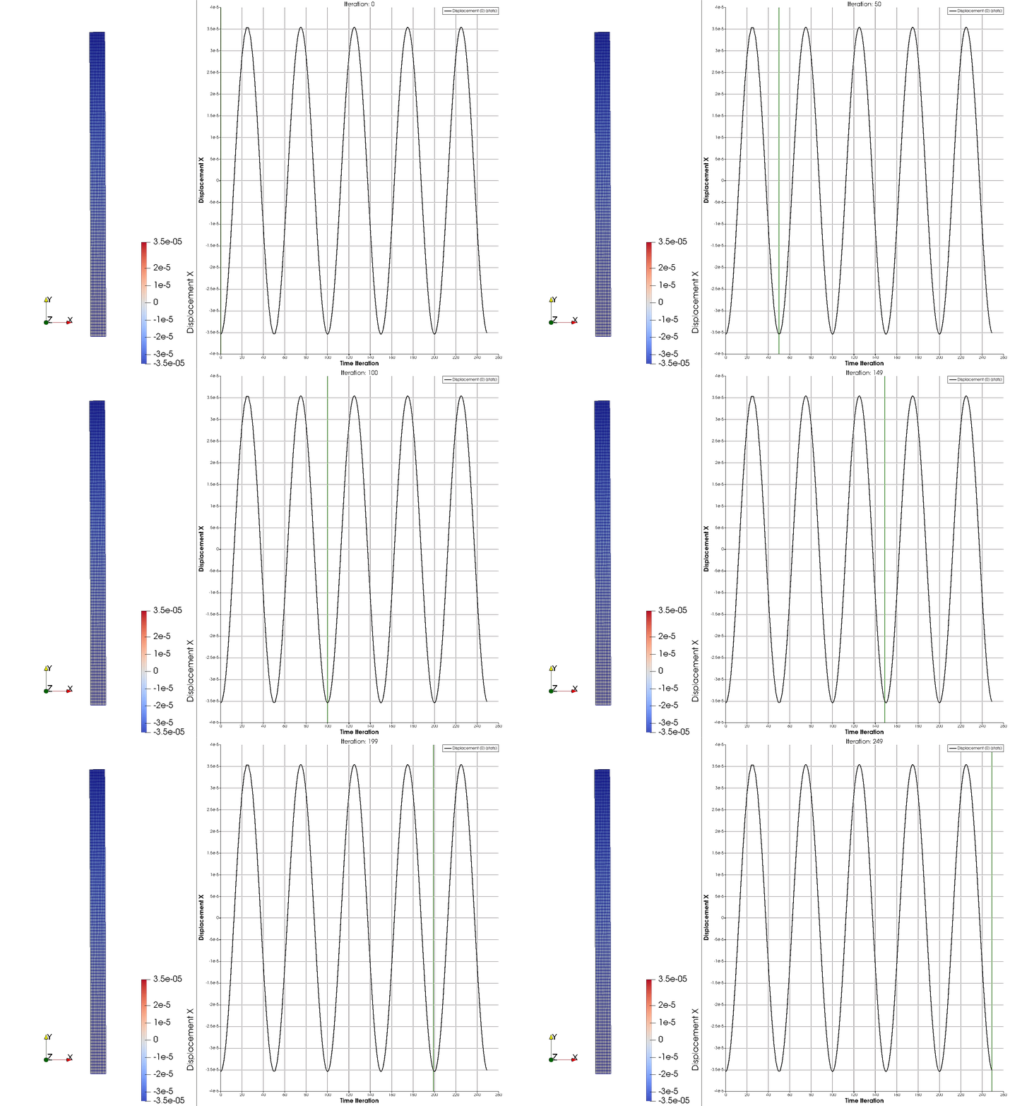
The solution of the problem is shown next, where the horizontal displacement at the tip is plotted on the right part of the figure, and the deformed configuration on the left.

References

\(^1\) Newmark, N.M. (1959), A method of computation for structural dynamics, J Eng Mech Div, 85(3):67-94

Attribution

If you are using this content for your research, please kindly cite the following reference (reference \(^2\) in the text above) in your derived works:

Sanchez, R. et al. (2016), Towards a Fluid-Structure Interaction solver for problems with large deformations within the open-source SU2 suite, 57th AIAA/ASCE/AHS/ASC Structures, Structural Dynamics, and Materials Conference, 4-8 January 2016, San Diego, California, USA. DOI: 10.2514/6.2016-0205

This work is licensed under a Creative Commons Attribution 4.0 International License