Non-ideal compressible flows with physics-informed neural networks

Goals

Upon completing this tutorial, the user will be familiar with performing simulations of nonideal compressible fluids through the use of physics-informed neural networks. The flow is simulated through the same supersonic convergent-divergent nozzle as in the tutorial for nonideal compressible fluid flows. The following capabilities of will be showcased in this tutorial:

• Using SU2 DataMiner to train physics-informed neural networks for fluid simulations.
• Data-driven equation of state with multi-layer perceptrons.
• Giles boundary conditions

The intent of this tutorial is to explain how to use the data-driven equation of state in SU2 for fluid simulations and how to train the neural network(s) required for modeling the fluid properties. The fluid used in this tutorial is Siloxane MM, but the methods explained in this tutorial can also be repeated for different fluids available within CoolProp.

Background

The data-driven equation of state in SU2 can be used to calculate the thermodynamic state properties of the fluid during CFD calculations. The method uses an equation of state based on entropy potential, allowing for the thermodynamic state variables to be directly calculated from the density and internal energy, which can be directly obtained from the solution of the flow transport equations.

The thermodynamic state variables are calculated from the Jacobian and Hessian of entropy w.r.t. density and internal energy. The data-driven fluid model in SU2 uses a physics-informed neural network to calculate the entropy Jacobian and Hessian such that thermodynamic consistency is maintained.

The data-driven, entropy-based equation of state is discussed more in detail in this paper.

Resources and Set-Up

You can find the resources for this tutorial in the folder compressible_flow/NICFD_nozzle/PhysicsInformed in the tutorial repository. You will need the python scripts and the nozzle contour file which describes the shape of the nozzle. The SU2 config file and mesh will be automatically generated using the scripts in this tutorial.

This tutorial requires SU2 DataMiner to run. Follow the installation instructions on the repository page, and install the required python packages. To be able to use the data-driven fluid model in SU2, compile SU2 with the following command:

meson.py build -Denable-mlpcpp=true

which will download the MLPCpp submodule enabling the evaluation of deep, dense multi-layer perceptrons in SU2.

Tutorial

The following steps explain how to train physics-informed neural networks for data-driven fluid simulations in SU2.

1. Generate SU2 DataMiner Configuration

Similar to SU2, SU2 DataMiner uses a configuration file to store information regarding the type of fluid, the resolution of the training data set, and the hyperparameters of the networks. Running the script 0:generate_config.py generates the SU2 DataMiner configuration used in this tutorial and is saved as a binary file named SU2DataMiner_MM.cfg.

2. Generate Training Data

The thermodynamic state data used to train the network for the data-driven fluid simulation is generated using the Helmholtz equation of state evalauted through the python module for CoolProp. The thermodynamic state data are generated on a density-static energy grid for the gas and supercritical phase between the minimum and maximum density of the fluid supported by CoolProp. The ranges for density and energy or pressure and temperature within which training data are generated can be manually specified.

By running the script 1:generate_fluid_data.py will generate the thermodynamic state data used for the training of the network and generate contour plots of the temperature, pressure, and speed of sound. The complete set of thermodynamic state data is stored in the file titled fluid_data_full.csv. 80% of the randomly sampled fluid data is used to update the weights of the network during training, 10% is used to monitor the convergence of the training process, and the remaining 10% is used to validate the accuracy of the network upon completion of the training process. The complete data set contains approximately 2.3e5 unique data points.

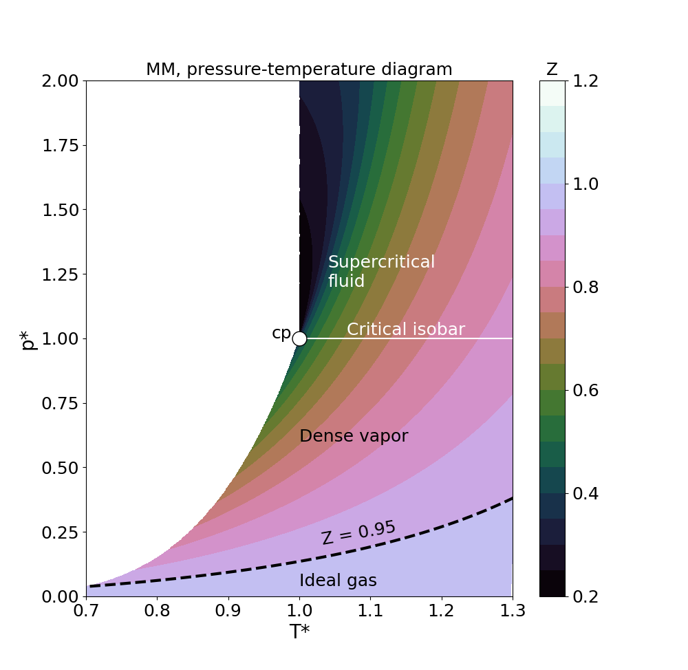Figure (1): Section of training data set near the critial point (‘cp’).

3. Train physics-informed neural network

The network used in this tutorial uses two hidden layers with 12 nodes each. The exponential function is used as the hidden layer activation function. This is an unusual choice, but is motivated by the fact that it reduces the computational cost required to calculate the network Jacobian and Hessian during the CFD solution process. The training process uses an exponential decay function for the learning rate, with an initial value of 1e-3. During each update step, the weights and biases of the network are adjusted according to the value of the loss function evaluated on a batch of 64 training data points. The hidden layer architecture and learning rate of the network used in this tutorial were selected through trial and error. More details regarding the training method are presented in the literature.

The training progress can be followed from the terminal, but can also be monitored from the training convergence plots that are periodically updated under Worker_0/Model_0/.

After training, the weights and biases of the network are stored in the SU2 DataMiner configuration.

IMAGE: training history plot, predicted vs training data

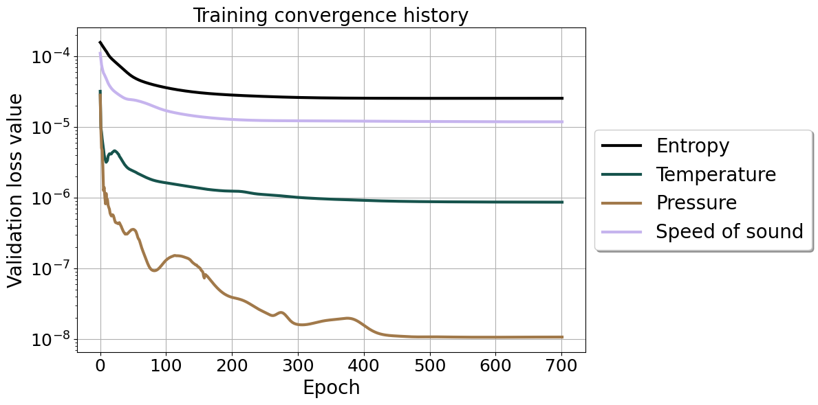Figure (2): Training convergence history

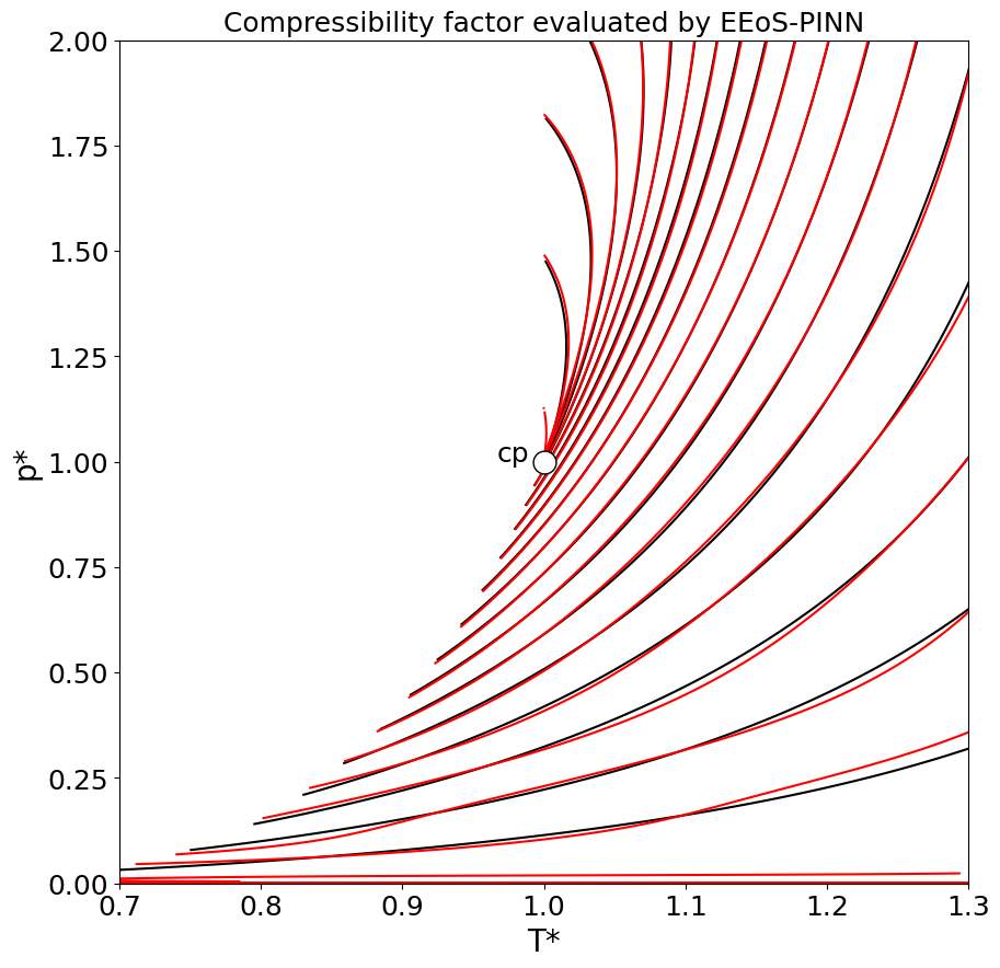Figure (3): Compressibility factor from reference data (black) and evaluated by data-driven equation of state (red).

4. Preparation of the Simulation

To run data-driven fluid simulations in SU2, you need the SU2 configuration file, the mesh, and the file describing the multilayer perceptron. Running the script 3:prepare_simulation.py generates the computational mesh, writes the SU2 configuration file, and writes the ASII file containing the weights and biases of the network.

The mesh is generated using gmesh in which the computational domain is generated accoring to the nozzle contour. The nozzle wall is modeled as a non-slip surface and prism layer refinement is applied to resolve the boundary layer.

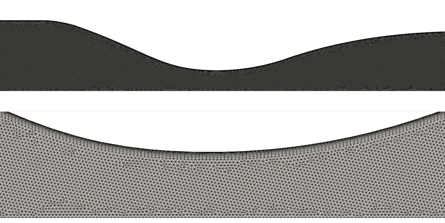Figure (4): Computational mesh used for the nozzle flow simulation (top) and highlight of the throat area near the wall (bottom).

The inflow condition is modeled as a non-reflective Giles boundary condition where the pressure and temperature of the critical point of the fluid are imposed as the stagnation pressure and stagnation temperature. The outflow is also modeled as a non-reflective Giles boundary condition, where a static pressure 10 times lower than the inflow pressure is imposed. To improve the stability of the solution process, the pressure imposed at the outflow boundary ramps down from the inflow stagnation pressure to the target value over the course of the first 200 flow iterations.

The data-driven fluid model with the physics-informed entropy-based equation of state is enabled through the following options in the SU2 configuration file:

FLUID_MODEL= DATADRIVEN_FLUID
USE_PINN= YES 
INTERPOLATION_METHOD= MLP
FILENAMES_INTERPOLATOR= MLP_siloxane_MM.mlp

where the USE_PINN= YES option enables the use of a physics-informed neural network for thermodynamic state calculations. The file MLP_siloxane_MM.mlp is the ASII file which describes the network architecture and the network weights and biases. At the start of the SU2 solution process, the network weigths and biases are imported into SU2 through the MLPCpp sub-module.

5. Run SU2

The simulation us run by the following command

mpirun -n <NP> SU2_CFD config_NICFD_PINN.cfg 

where <NP> is the number of cores. Figure 5 shows the residual trends of the flow solution of the course of 10k iterations.

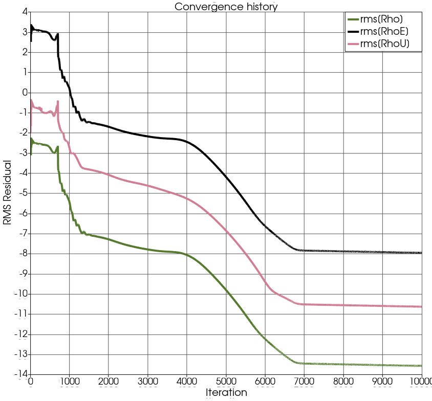Figure (5): Convergence history of the SU2 simulation.

Results

The Mach number and compressibility factor of the flow solution is visualized in the image below. The flow expands to supersonic speeds in the divergent section of the nozzle, where the compressibility factor approaches a value of 1.0, while the compressibility factor is significantly lower in the convergent section of the nozzle. 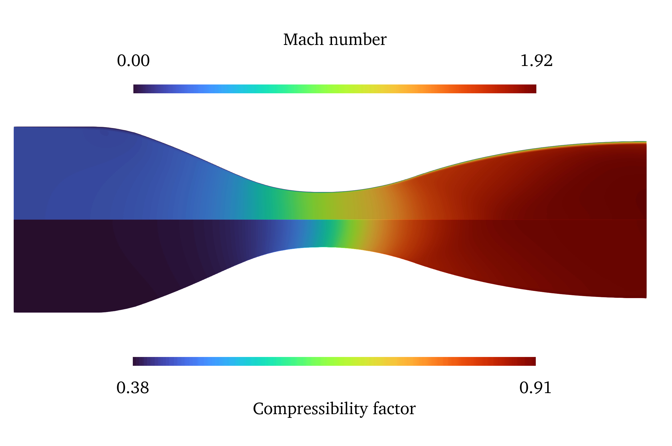Figure (6): Mach number of the flow solution (top) and compressibility factor of the fluid (bottom).