-
Inviscid Bump in a Channel
Inviscid Supersonic Wedge
Inviscid ONERA M6
Laminar Flat Plate
Laminar Cylinder
Turbulent Flat Plate
Transitional Flat Plate
Transitional Flat Plate for T3A and T3A-
Turbulent ONERA M6
Unsteady NACA0012
Epistemic Uncertainty Quantification of RANS predictions of NACA 0012 airfoil
Non-ideal compressible flow in a supersonic nozzle
Non-ideal compressible flows with physics-informed neural networks
Aachen turbine stage with Mixing-plane
-
Inviscid Hydrofoil
Laminar Flat Plate with Heat Transfer
Turbulent Flat Plate
Turbulent NACA 0012
Laminar Backward-facing Step
Laminar Buoyancy-driven Cavity
Streamwise Periodic Flow
Species Transport
Composition-Dependent model for Species Transport equations
Unsteady von Karman vortex shedding
Turbulent Bend with wall functions
Wind velocity and pollutant dispersion in a city
-
Static Fluid-Structure Interaction (FSI)
Dynamic Fluid-Structure Interaction (FSI) using the Python wrapper and a Nastran structural model
Static Conjugate Heat Transfer (CHT)
Unsteady Conjugate Heat Transfer
Solid-to-Solid Conjugate Heat Transfer with Contact Resistance
Incompressible, Laminar Combustion Simulation
User Defined combustion model with Python
-
Unconstrained shape design of a transonic inviscid airfoil at a cte. AoA
Constrained shape design of a transonic turbulent airfoil at a cte. CL
Constrained shape design of a transonic inviscid wing at a cte. CL
Shape Design With Multiple Objectives and Penalty Functions
Unsteady Shape Optimization NACA0012
Unconstrained shape design of a two way mixing channel
Adjoint design optimization of a turbulent 3D pipe bend
Unsteady NACA0012
| Written by | for Version | Revised by | Revision date | Revised version |
|---|---|---|---|---|
| @ScSteffen | 7.0.1 | @talbring | 2020-03-03 | 7.0.2 |
Solver: |
|
Uses: |
|
Prerequisites: |
None |
Complexity: |
Basic |
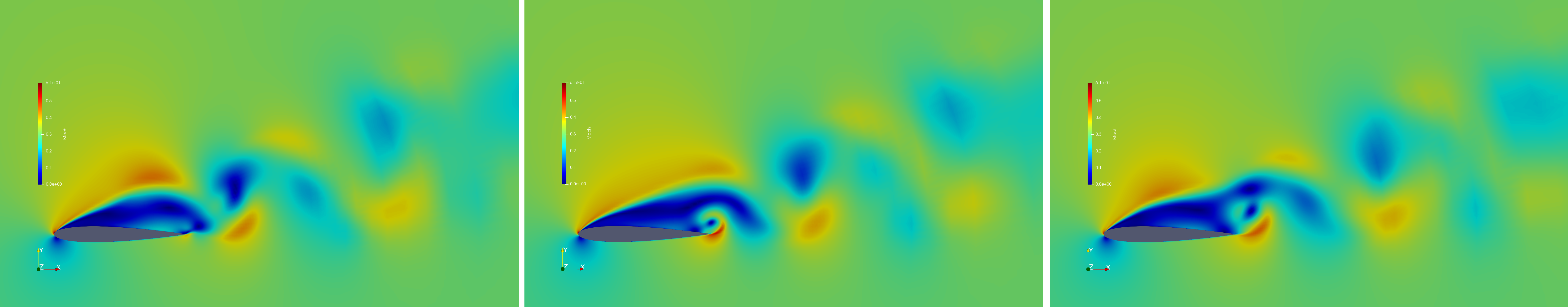 Figure (1): An unsteady, periodic flow field. The detached flow about the airfoil results in a vortex street that repeats itself after some time.
Goals
Upon completing this tutorial, the user will be familiar with performing a simulation of external, viscous, unsteady periodic flows around a 2D geometry using a turbulence model. The specific geometry chosen for the tutorial is the classic NACA0012 airfoil. Furthermore, the user is introduced in the so-called windowing approach, a regularizing method for time averaging in unsteady periodic flows. Consequently, the following capabilities of SU2 will be showcased in this tutorial:
- Unsteady, 2D URANS equations
- Dual time-stepping for unsteady flows
- Windowing
- Time-convergence
This tutorial also provides an explanation for properly setting up viscous, compressible, unsteady 2D flow conditions in SU2. We also introduce a new type of time-convergence criteria for periodic flows, which monitors the change of the time-average of a specific objective, such as lift or drag, in order to assess convergence.
Resources
The resources for this tutorial can be found in the compressible_flow/Unsteady_NACA0012 directory in the tutorials website repository. You will need the configuration file (unsteady_naca0012.cfg) and the mesh file (unsteady_naca0012_mesh.su2) as well as the restart files (restart_flow_00497.dat, restart_flow_00498.dat, restart_flow_00499.dat).
Tutorial
The following tutorial will walk you through the steps required when solving for the flow about the NACA0012 airfoil using SU2. The tutorial will also address procedures for both serial and parallel computations. To this end, it is assumed you have already obtained and compiled SU2_CFD. If you have yet to complete these requirements, please see the Download and Installation pages.
Background
This test case is for the NACA0012 airfoil in viscous unsteady flow. The NACA airfoils are two dimensional shapes for aircraft wings developed by the National Advisory Committee for Aeronautics (NACA, 1915-1958, predeccessor of NASA). The NACA-4-Digit series is a set of 78 airfoil configurations, which were created for wind-tunnel tests to explore the effect of different airfoil shapes on aerdynamic coefficients as drag or lift.
Problem Setup
This problem will solve the flow about the airfoil with these conditions:
- Freestream Temperature = 293.0 K
- Freestream Mach number = 0.3
- Angle of attack (AOA) = 17.0 deg
- Reynolds number = 1E3
- Reynolds length = 1.0 m
These subsonic flow conditions cause a detached flow on the upper side of the airfoil, which result in a vortex street and therefore periodic behavior.
Mesh Description
The computational domain consists of a grid of 14495 quadrilaterals, that sourrounds the NACA0012 airfoil. Note that this is a very coarse mesh, and should one wish to obtain more accurate solutions for comparison with results in the literature, finer grids should be used.
Two boundary conditions are employed: the Navier-Stokes adiabatic wall condition on the wing surface and the far-field characteristic-based condition on the far-field marker.
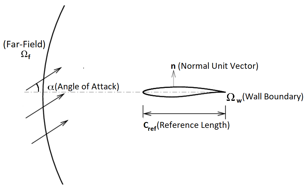 Figure (2): Far-field view of the computational domain.
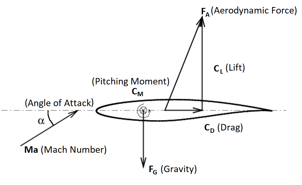 Figure (3): Close-up view of the airfoil surface and the aerodynamic coefficients.
Configuration File Options
Configuration of the physical problem is similar to the ONERA M6 tutorial, that one can access here. However, contrary to the ONERA M6 case, here an unsteady simulation is performed, hence, the Unsteady RANS (URANS) equations in 2D must be solved. Unsteady RANS simulations in SU2 are typically computed via the dual time-stepping approach. To this end, one first performs a spatial discretization as explained in the ONERA M6 tutorial. After that, a time discretization in physical time is performed, that results in a residual equation of the form
\[R(u^n) = 0 \qquad \forall n=1,\dots,N.\]Here, \(n\) denotes the current physical time iteration, \(N\) is the final (physical) time of the simulation, and \(R\) is the residual, one has to solve. In this tutorial, a second order BDF scheme is employed. The idea of dual time-stepping is, that the current solution \(u^n\) of the residual equation is computed for each time step by solving an ordinary differential equation in pseudo time \(\tau\). The ODE for physical time-step \(n\) reads
\[\partial_\tau u^n + R(u^n) = 0.\]Now, a steady state solution for this ODE is computed using the steady state solver. Once a solution is aquired, the residual equation for the next physical time step \(n+1\) is set up.
As a result there are two time iterators. The inner (pseudo time) iterator and the outer (physical time) iterator. The number of iterations for the pseudo time iterator is specified by INNER_ITER and the number of iterations
for the physical time iterator by TIME_ITER. The option TIME_DOMAIN=YES activates the time dependent solver in SU2.
The option TIME_MARCHING specifies the numerical method to discretize the time domain in physical time and TIME_STEP
denotes the length of the physical time-step used.
The numerical method to solve the inner (pseudo time) ODE is given by the option TIME_DISCRE_FLOW.
% -------------UNSTEADY SIMULATION ----------------%
%
TIME_DOMAIN = YES
%
% Numerical Method for Unsteady simulation
TIME_MARCHING= DUAL_TIME_STEPPING-2ND_ORDER
%
% Time Step for dual time stepping simulations (s)
TIME_STEP= 5e-4
%
% Maximum Number of physical time steps.
TIME_ITER= 2000
%
% Number of internal iterations (dual time method)
INNER_ITER= 10
%
% Time discretization for inner iteration.
TIME_DISCRE_FLOW= EULER_IMPLICIT
%
This unsteady simulation results in a periodic flow, which can be seen by the vortex street in the flow visualization above. However, since the initial conditions are set to free-stream conditions, a couple of iterations are needed to reach the periodic state. This time-span is called transient phase.
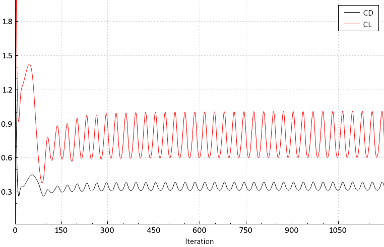 Figure (4): Time-dependent drag (black) and lift (red) coefficient. The transient time spans approximately 300 (physical) time-steps.
Usually in a periodic flow an instantaneous output value, e.g. \(C_D(t)\), is not meaningful. Hence one often uses the average value of one period \(T\):
\[\frac{1}{T}\int_0^T C_D(t) \mathcal{d}t\]However, the exact duration of a period is unknown or cannot be resolved due to a too coarse time discretization. Therefore, one averages over a finite time-span \(M\), which lasts a couple of periods and hopes for convergence to the period-average
\[\frac{1}{M}\int_0^M C_D(t) \mathcal{d}t.\]If one employs a weighting function \(w(t)\), called window-function, the time-average converges faster to the actual period-average
\[\frac{1}{M}\int_0^M w(t/M)C_D(t) \mathcal{d}t.\]A windowing function is a function, that is zero on its boundaries \(0\) and \(M\) and has integral \(1\). The iteration
to start the windowed time-average is specified with WINDOW_START_ITER. Note, that at this iteration the transient phase of the flow must have passed. Otherwise a time average that approximates a period average is not meaningful.
The windowing function can be specified with the option WINDOW_FUNCTION.
Note, that windowing functionality also works for sensitivities of time dependent outputs. In this case, the order of convergence is reduced by 1.
The following options are implemented:
| Window | Convergence Order | Convergence Order (sensitivity) |
|---|---|---|
SQUARE |
1 | 0 |
HANN |
3 | 2 |
HANN_SQUARE |
5 | 4 |
BUMP |
exponential | exponential |
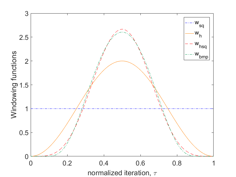 Figure (5): Different window-functions in the time span from 0 to 1.
The SQUARE-window denotes the case of uniform weighting by 1, i.e. the case, where no windowing-function is applied. It is not recommended to use SQUARE- windowing for sensitivities, since no convergence is guaranteed.
For further information about the windowing approach, we refer to the work of Krakos et al. (Sensitivity Analysis of Limit Cycle Oscillations).
The windowed time-averaged output-field can be accessed in SCREEN_OUTPUT by adding the prefix TAVG_ to the chosen output-field. For
time-averaged sensitivities, one adds the prefix D_TAVG_.
The windowing functionality can also be used to monitor time convergence. Similar to the steady-state case, a Cauchy-criterion can be employed for flow coefficients.
The Cauchy-criterion is applied to the windowed time-average from the iteration specified by WINDOW_START_ITER + CONV_WINDOW_STARTITER up to the current iteration.
The field or the list of fields to be monitored can be specified by CONV_WINDOW_FIELD.
The solver will stop, if the average over a certain number of elements (set with CONV_WINDOW_CAUCHY_ELEMS) is smaller than the value set with CONV_WINDOW_CAUCHY_EPS.
The windowed time-averaged Cauchy criterion can be activated by setting WINDOW_CAUCHY_CRIT = YES (default is NO).
If a list of multiple convergence fields is chosen, the sovlver terminates, if the Cauchy criterion is satisfied for all fields in the list.
% --- Coefficient-based Windowed Time Convergence Criteria ----%
%
% Activate the windowed cauchy criterion
WINDOW_CAUCHY_CRIT = YES
%
% Specify convergence field(s)
CONV_WINDOW_FIELD= (TAVG_DRAG, TAVG_LIFT)
%
% Number of elements to apply the criteria
CONV_WINDOW_CAUCHY_ELEMS= 10
%
% Epsilon to control the series convergence
CONV_WINDOW_CAUCHY_EPS= 1E-4
%
% Number of iterations to wait after the iteration specified in  WINDOW_START_ITER.
CONV_WINDOW_STARTITER = 10
%
% Iteration to start the windowed time average
WINDOW_START_ITER = 500
%
% Window-function to weight the time average. Options (SQUARE, HANN, HANN_SQUARE, BUMP), SQUARE is default.
WINDOW_FUNCTION = HANN_SQUARE
Usually a case is not purely periodic, but the period-mean has a slight shift upwards or downwards. Hence, the time-convergence epsilon value is typically not as small as in the time-steady case.
As one can see in Fig. (4), the transient phase of drag (and lift) is about 500 iterations, thus a suitable starting time for the windowed-average is WINDOW_START_ITER=500.
To skip the transient phase (and speed up the tutorial a bit), a restart solution is provided.
% Restart after the transient phase has passed
RESTART_SOL = YES
%
% Specify unsteady restart iter
RESTART_ITER = 499
Running SU2
The airfoil mesh should fit on a single-core machine. To run this test case follow these steps at a terminal command line:
- Move to the directory containing the config file (unsteady_naca0012.cfg) and the mesh file (unsteady_naca0012_mesh.su2). Make sure that the SU2 tools were compiled, installed, and that their install location was added to your path.
- For serial execution run the command:
$ SU2_CFD unsteady_NACA0012.cfg - SU2 will print residual updates with each iteration of the flow solver, and the simulation will terminate after reaching the specified convergence criteria.
- Files containing the results will be written on every time step.
To run the case in parallel (using MPI) simply do:
$ mpirun -n NP SU2_CFD unsteady_NACA0012.cfg
Where NP is the number of processors, note that different MPI distributions may need slightly different syntax (e.g. mpiexec).
Results
Results for the flow about the NACA0012 airfoil are shown below. The first picture shows the time dependent drag (black) as well as the windowed average from iteration 500 up to the current iteration computed with different windowing-functions. The Hann-Square-windowed time-average set up in this tutorial is displayed by the red line. The simulation terminates at iteration 532, since then, the Cauchy time-convergence criteria are satisfied. The second picture shows a simulation, where the convergence criterion is deactivated. Note, that the Square-window oscillates much longer than the other windows, due to its low convergence order.
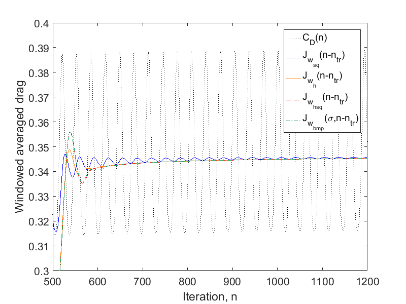
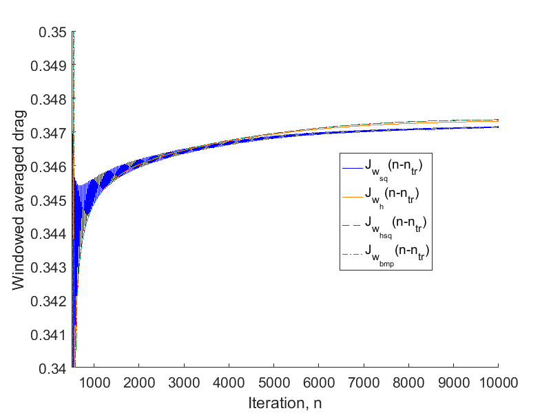
Figure (6): Comparison of time-averages using different window-functions